Objectives To describe a programming language we call

Objectives: ❑ To describe a programming language we call Simple Language and define its basic statements. ❑ To write macros in Simple Language using the combination of simple statements. ❑ To describe the components of a Turing machine as a computation model. ❑ To show simple statements in Simple Language can be simulated using a Turing machine. ❑ To understand the Church-Turing thesis and its implication.

Objectives (continued): ❑ To define the Gödel number and its application. ❑ To understand the concept of the halting problem and how it can be proved that this problem is unsolvable. ❑ To distinguish between solvable and unsolvable problems. ❑ To distinguish between polynomial solvable problems. and non-

17. 1 INTRODUCTION This chapter is a brief introduction to theory of computation. First, we introduce a language we call Simple Language, to show that the minimum number of statements needed to solve any problem that is solvable by a computer is three. Second, we explain another tool, a computer model called the Turing machine. We show that a problem that can be solved by our Simple Language can also be solved by the Turing machine.

17. 1 INTRODUCTION (Continued) Third, we prove that no program can tell whether another program halts or not. This proof is itself an indication that there are problems that cannot be solved by a computer. Finally, we briefly discuss the complexity of algorithms.

17. 2 SIMPLE LANGUAGE We can define a computer language with only three statements: the increment statement, the decrement statement, and the loop statement. In this language, the only data type we use is nonnegative integers. There is no need for any other data type, because the goal of the chapter is merely to demonstrate some ideas in computation theory.

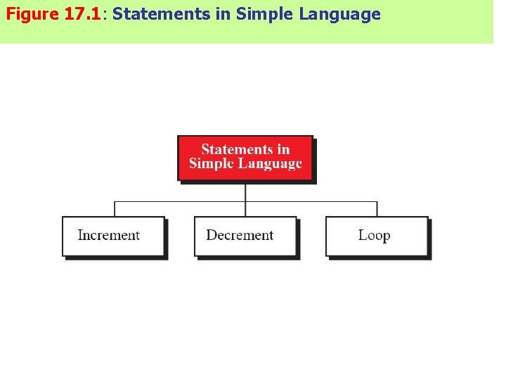
Figure 17. 1: Statements in Simple Language

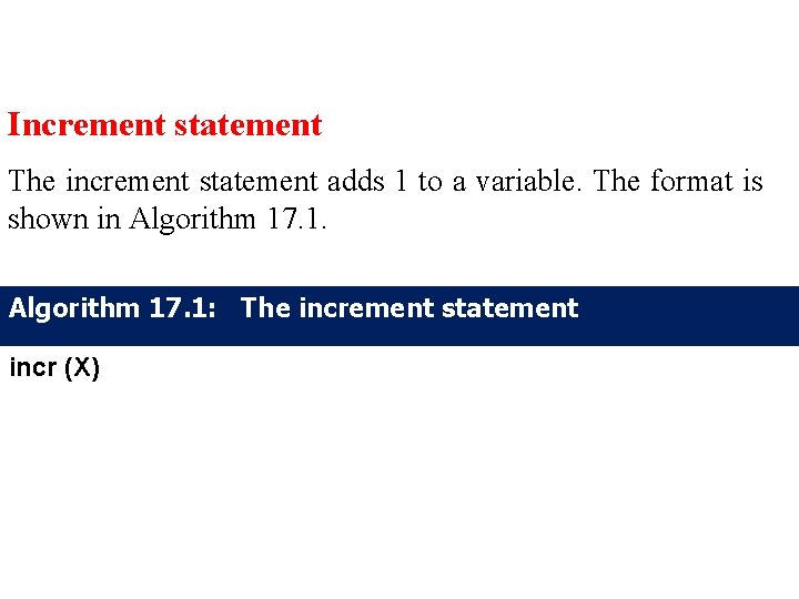
Increment statement The increment statement adds 1 to a variable. The format is shown in Algorithm 17. 1: The increment statement incr (X)

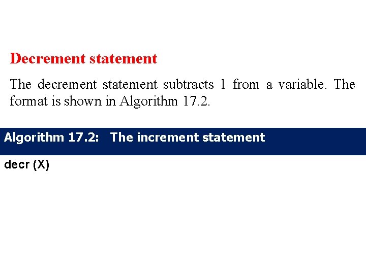
Decrement statement The decrement statement subtracts 1 from a variable. The format is shown in Algorithm 17. 2: The increment statement decr (X)

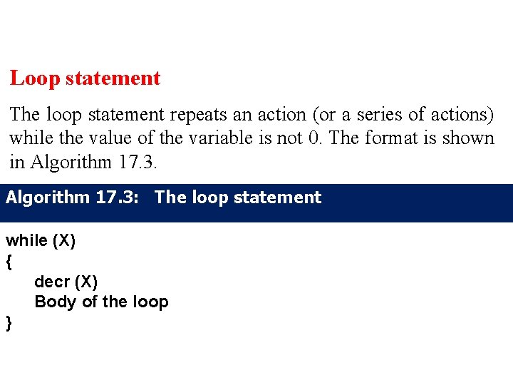
Loop statement The loop statement repeats an action (or a series of actions) while the value of the variable is not 0. The format is shown in Algorithm 17. 3: The loop statement while (X) { decr (X) Body of the loop }

The power of the Simple Language It can be shown that this simple programming language with only three statements is as powerful—although not necessarily as efficient—as any sophisticated language in use today, such as C. To do so, we show we can simulate several statements found in some popular languages. Macros in Simple Language We call each simulation a macro and use it in other simulations without the need to repeat code. A macro (short for macroinstruction) is an instruction in a high-level language that is equivalent to a specific set of one or more ordinary instructions in the same language.

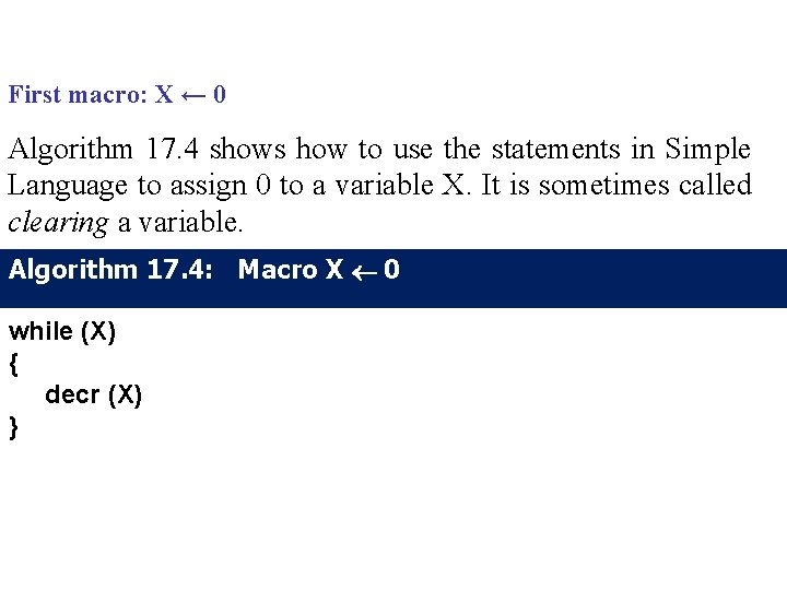
First macro: X ← 0 Algorithm 17. 4 shows how to use the statements in Simple Language to assign 0 to a variable X. It is sometimes called clearing a variable. Algorithm 17. 4: Macro X ¬ 0 while (X) { decr (X) }

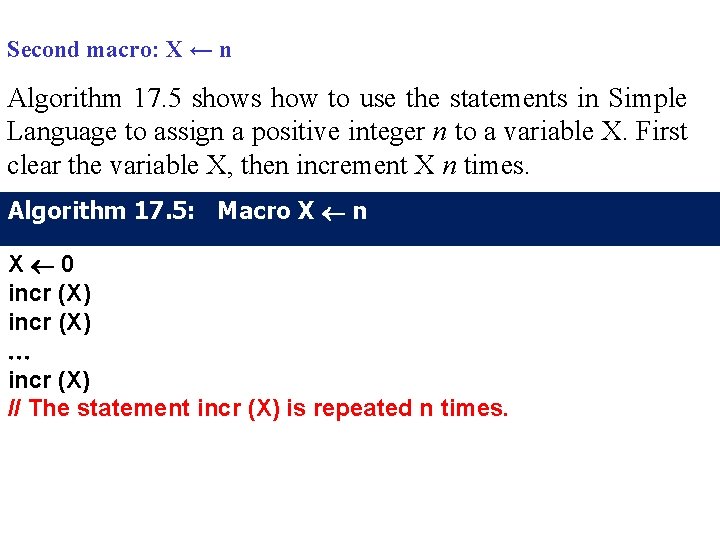
Second macro: X ← n Algorithm 17. 5 shows how to use the statements in Simple Language to assign a positive integer n to a variable X. First clear the variable X, then increment X n times. Algorithm 17. 5: Macro X ¬ n X¬ 0 incr (X) ¼ incr (X) // The statement incr (X) is repeated n times.

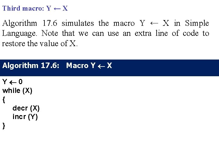
Third macro: Y ← X Algorithm 17. 6 simulates the macro Y ← X in Simple Language. Note that we can use an extra line of code to restore the value of X. Algorithm 17. 6: Macro Y ¬ X Y¬ 0 while (X) { decr (X) incr (Y) }

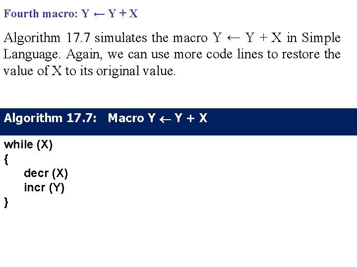
Fourth macro: Y ← Y + X Algorithm 17. 7 simulates the macro Y ← Y + X in Simple Language. Again, we can use more code lines to restore the value of X to its original value. Algorithm 17. 7: Macro Y ¬ Y + X while (X) { decr (X) incr (Y) }

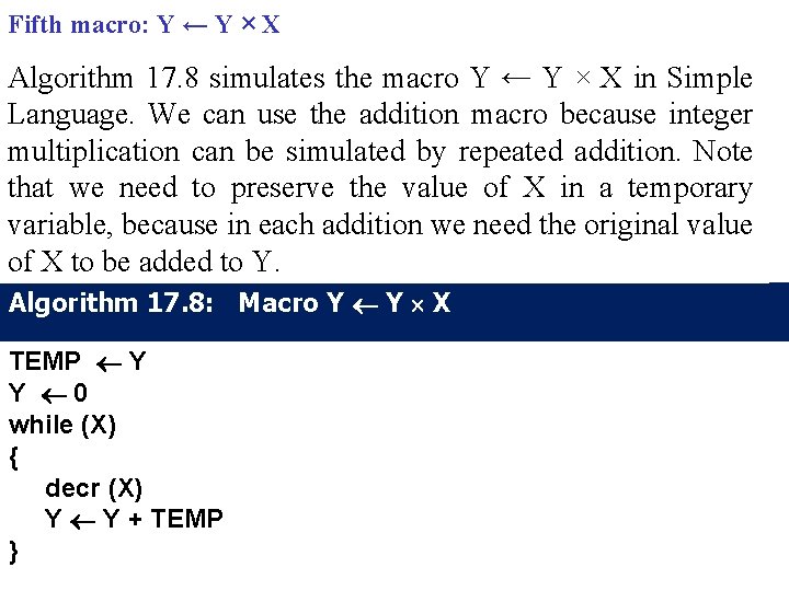
Fifth macro: Y ← Y × X Algorithm 17. 8 simulates the macro Y ← Y × X in Simple Language. We can use the addition macro because integer multiplication can be simulated by repeated addition. Note that we need to preserve the value of X in a temporary variable, because in each addition we need the original value of X to be added to Y. Algorithm 17. 8: Macro Y ¬ Y X TEMP ¬ Y Y ¬ 0 while (X) { decr (X) Y ¬ Y + TEMP }

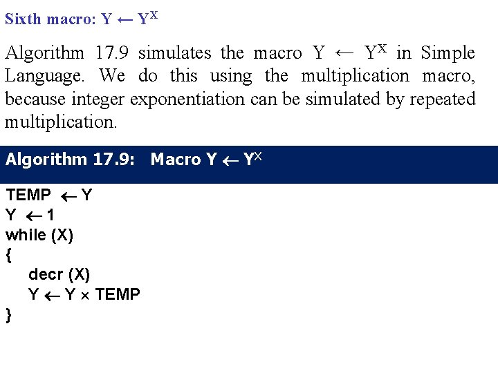
Sixth macro: Y ← YX Algorithm 17. 9 simulates the macro Y ← YX in Simple Language. We do this using the multiplication macro, because integer exponentiation can be simulated by repeated multiplication. Algorithm 17. 9: Macro Y ¬ YX TEMP ¬ Y Y ¬ 1 while (X) { decr (X) Y ¬ Y TEMP }

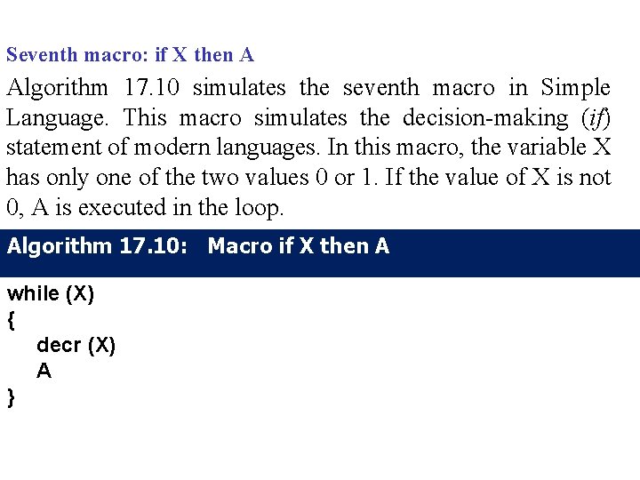
Seventh macro: if X then A Algorithm 17. 10 simulates the seventh macro in Simple Language. This macro simulates the decision-making (if) statement of modern languages. In this macro, the variable X has only one of the two values 0 or 1. If the value of X is not 0, A is executed in the loop. Algorithm 17. 10: Macro if X then A while (X) { decr (X) A }

Other macros It is obvious that we need more macros to make Simple Language compatible with contemporary languages. Creating other macros is possible, although not trivial. Input and output In this simple language the statement read X can be simulated using (X ← n). We also simulate the output by assuming that the last variable used in a program holds what should be printed. Remember that this is not a practical language, it is merely designed to prove some theorems in computer science.

17. 3 THE TURING MACHINE The Turing machine was introduced in 1936 by Alan M. Turing to solve computable problems, and is the foundation of modern computers. In this section we introduce a very simplified version of the machine to show it works.

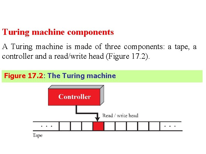
Turing machine components A Turing machine is made of three components: a tape, a controller and a read/write head (Figure 17. 2). Figure 17. 2: The Turing machine

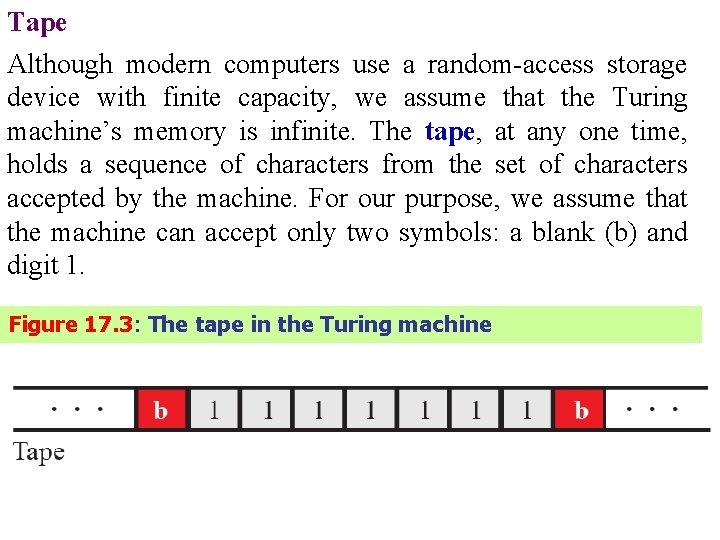
Tape Although modern computers use a random-access storage device with finite capacity, we assume that the Turing machine’s memory is infinite. The tape, at any one time, holds a sequence of characters from the set of characters accepted by the machine. For our purpose, we assume that the machine can accept only two symbols: a blank (b) and digit 1. Figure 17. 3: The tape in the Turing machine

Read/write head The read/write head at any moment points to one symbol on the tape. We call this symbol the current symbol. The read/write head reads and writes one symbol at a time from the tape. After reading and writing, it moves to the left or to the right. Reading, writing and moving are all done under instructions from the controller. Controller The controller is theoretical counterpart of the central processing unit (CPU) in modern computers. It is a finite state automaton, a machine that has a predetermined finite number of states and moves from one state to another based on the input.

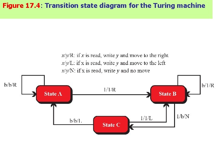
Figure 17. 4: Transition state diagram for the Turing machine

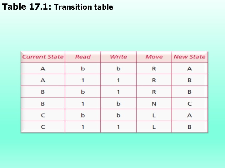
Table 17. 1: Transition table

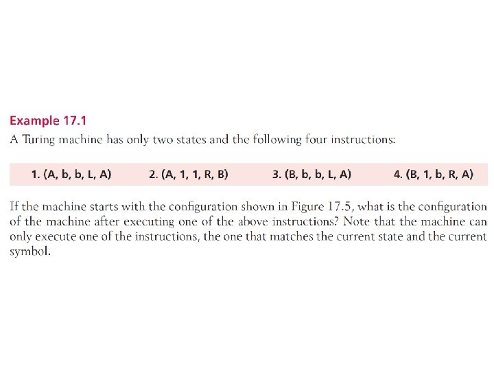
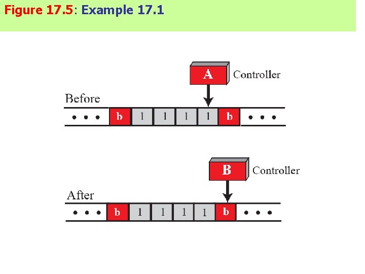
Figure 17. 5: Example 17. 1

Simulating Simple Language We can now write programs that implement the statements of Simple Language. Note that these statements can be written in many different ways: we have chosen the simplest or most convenient for our educational purpose, but they are not necessarily the best ones. Increment statement Figure 17. 6 shows the Turing machine for the incr(X) statement. The controller has four states, S 1 through S 4. State S 1 is the starting state, state S 2 is the moving-right state, state S 3 is the moving-left state and state 4 is the halting state.

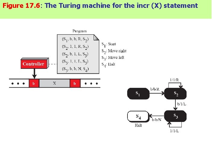
Figure 17. 6: The Turing machine for the incr (X) statement

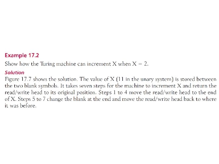
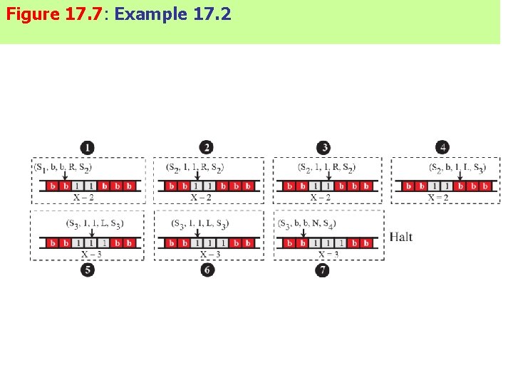
Figure 17. 7: Example 17. 2

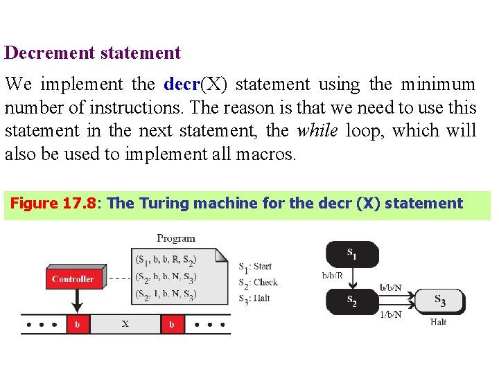
Decrement statement We implement the decr(X) statement using the minimum number of instructions. The reason is that we need to use this statement in the next statement, the while loop, which will also be used to implement all macros. Figure 17. 8: The Turing machine for the decr (X) statement

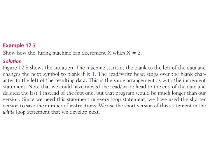
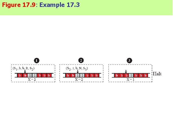
Figure 17. 9: Example 17. 3

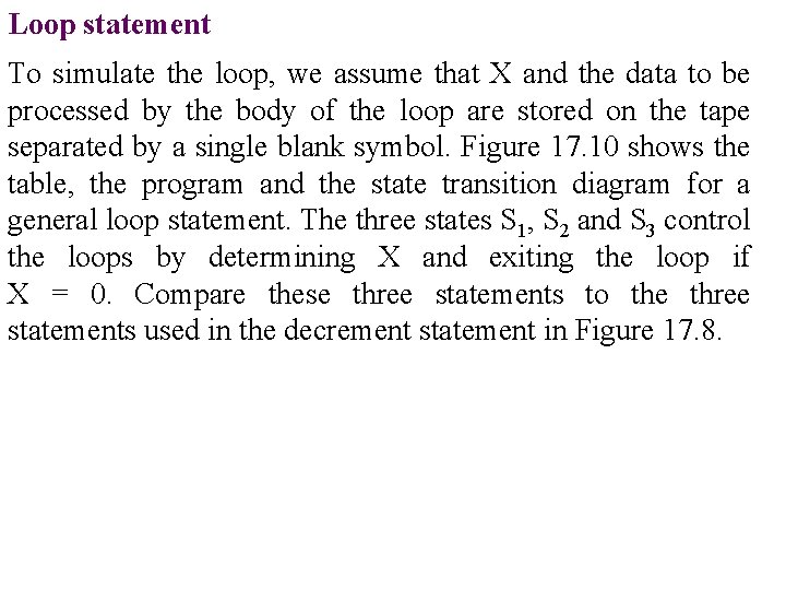
Loop statement To simulate the loop, we assume that X and the data to be processed by the body of the loop are stored on the tape separated by a single blank symbol. Figure 17. 10 shows the table, the program and the state transition diagram for a general loop statement. The three states S 1, S 2 and S 3 control the loops by determining X and exiting the loop if X = 0. Compare these three statements to the three statements used in the decrement statement in Figure 17. 8.

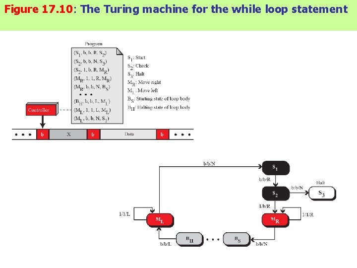
Figure 17. 10: The Turing machine for the while loop statement

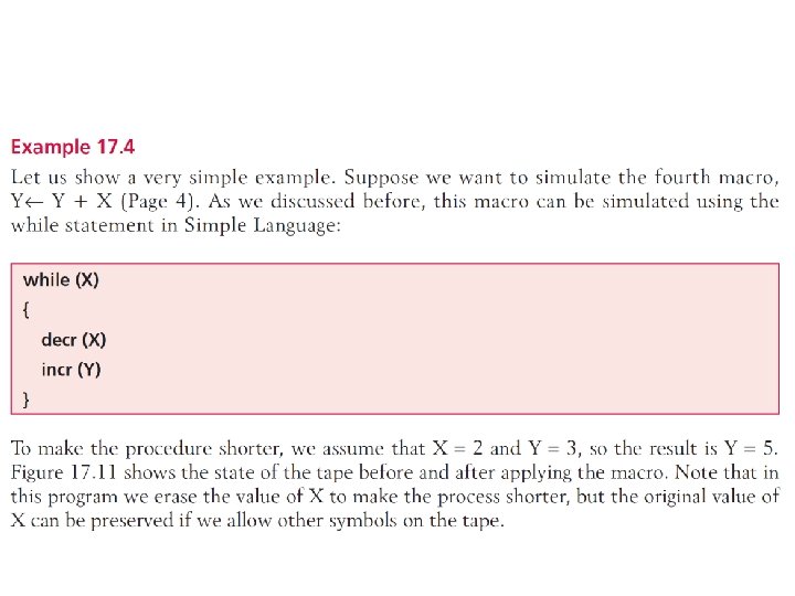
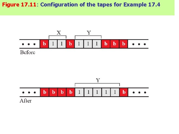
Figure 17. 11: Configuration of the tapes for Example 17. 4

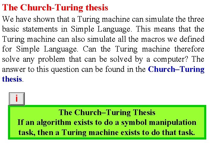
The Church-Turing thesis We have shown that a Turing machine can simulate three basic statements in Simple Language. This means that the Turing machine can also simulate all the macros we defined for Simple Language. Can the Turing machine therefore solve any problem that can be solved by a computer? The answer to this question can be found in the Church–Turing thesis. i The Church–Turing Thesis If an algorithm exists to do a symbol manipulation task, then a Turing machine exists to do that task.

17. 4 GODEL NUMBERS In theoretical computer science, an unsigned number is assigned to every program that can be written in a specific language. This is usually referred to as the Gödel number, named after the Austrian mathematician Kurt Gödel.

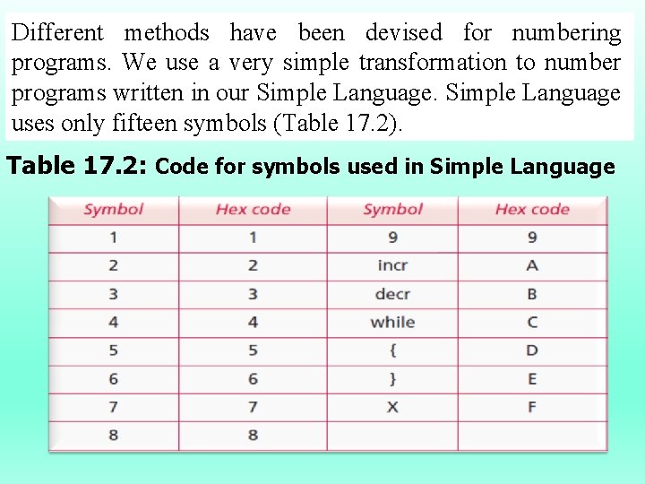
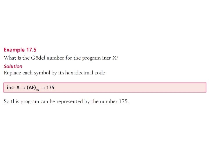
Different methods have been devised for numbering programs. We use a very simple transformation to number programs written in our Simple Language uses only fifteen symbols (Table 17. 2). Table 17. 2: Code for symbols used in Simple Language

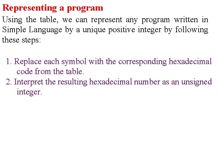
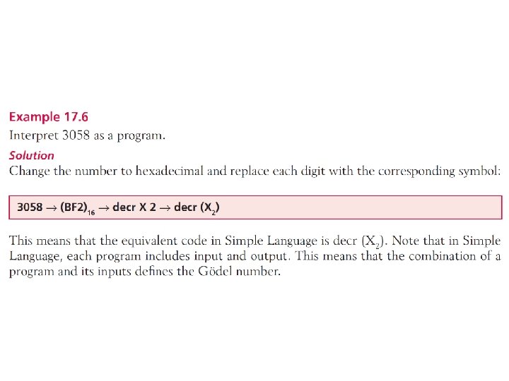
Representing a program Using the table, we can represent any program written in Simple Language by a unique positive integer by following these steps: 1. Replace each symbol with the corresponding hexadecimal code from the table. 2. Interpret the resulting hexadecimal number as an unsigned integer.

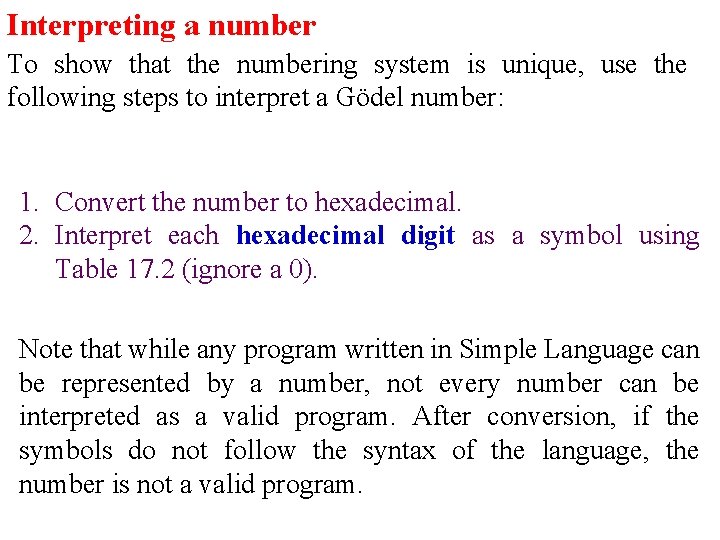
Interpreting a number To show that the numbering system is unique, use the following steps to interpret a Gödel number: 1. Convert the number to hexadecimal. 2. Interpret each hexadecimal digit as a symbol using Table 17. 2 (ignore a 0). Note that while any program written in Simple Language can be represented by a number, not every number can be interpreted as a valid program. After conversion, if the symbols do not follow the syntax of the language, the number is not a valid program.

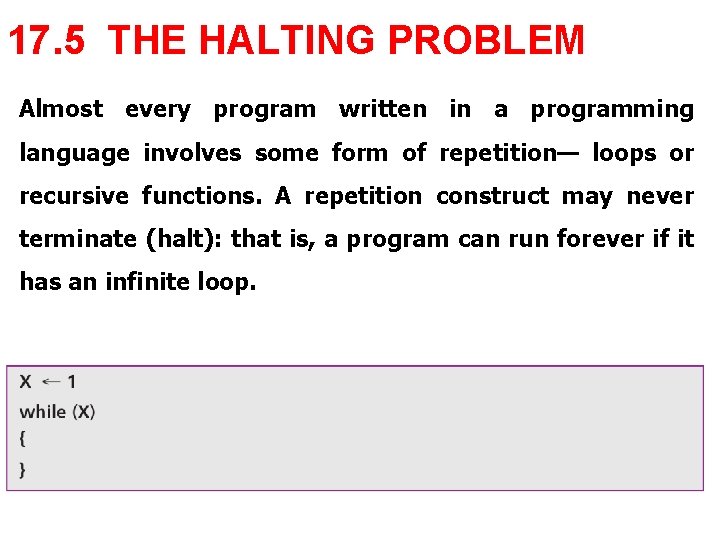
17. 5 THE HALTING PROBLEM Almost every program written in a programming language involves some form of repetition— loops or recursive functions. A repetition construct may never terminate (halt): that is, a program can run forever if it has an infinite loop.

A classical programming question is: i Can we write a program that tests whether or not any program, represented by its Gödel number, will terminate? The existence of this program would save programmers a lot of time. Running a program without knowing if it halts or not is a tedious job. Unfortunately, it has now been proven that such a program cannot exist—much to the disappointment of programmers!

The halting problem is not solvable Instead of saying that the testing program does not exist and can never exist, the computer scientist says “The halting problem is not solvable”. Proof Let us give an informal proof about the nonexistence of this testing program. Our method, called proof by contradiction, is often used in mathematics: we assume that the program does exist, then show that its existence creates a contradiction—therefore, it cannot exist. We use three steps to show the proof in this approach.

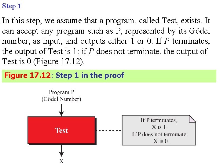
Step 1 In this step, we assume that a program, called Test, exists. It can accept any program such as P, represented by its Gödel number, as input, and outputs either 1 or 0. If P terminates, the output of Test is 1: if P does not terminate, the output of Test is 0 (Figure 17. 12). Figure 17. 12: Step 1 in the proof

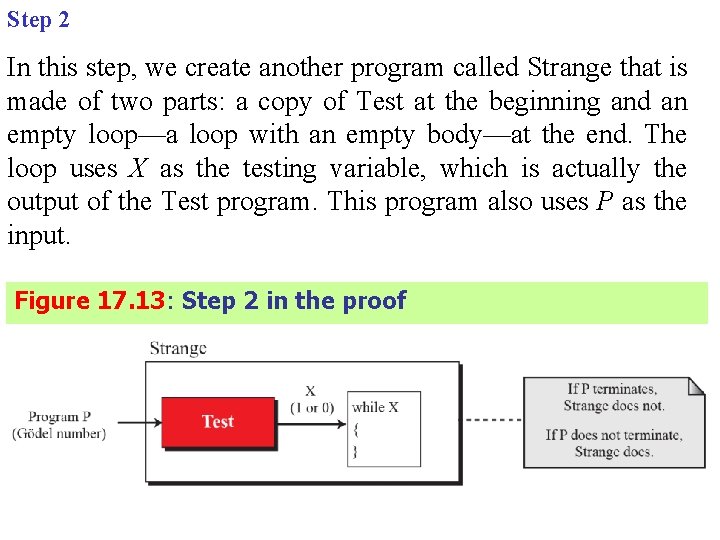
Step 2 In this step, we create another program called Strange that is made of two parts: a copy of Test at the beginning and an empty loop—a loop with an empty body—at the end. The loop uses X as the testing variable, which is actually the output of the Test program. This program also uses P as the input. Figure 17. 13: Step 2 in the proof

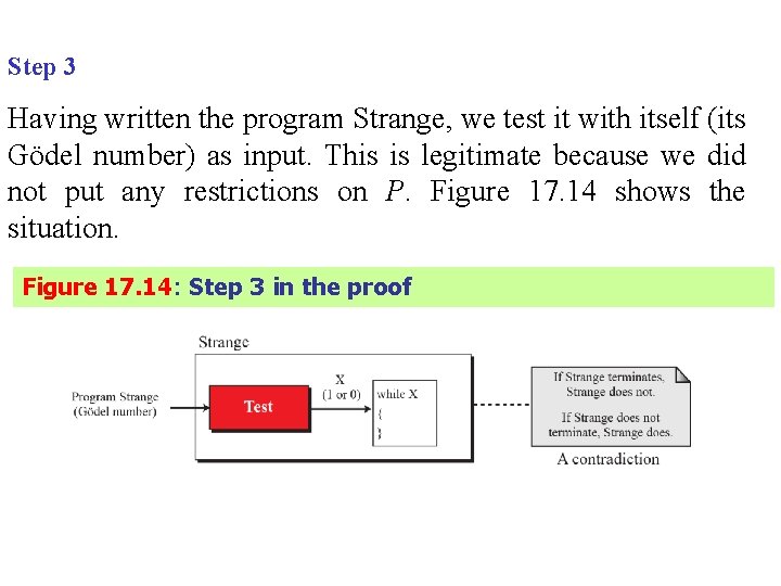
Step 3 Having written the program Strange, we test it with itself (its Gödel number) as input. This is legitimate because we did not put any restrictions on P. Figure 17. 14 shows the situation. Figure 17. 14: Step 3 in the proof

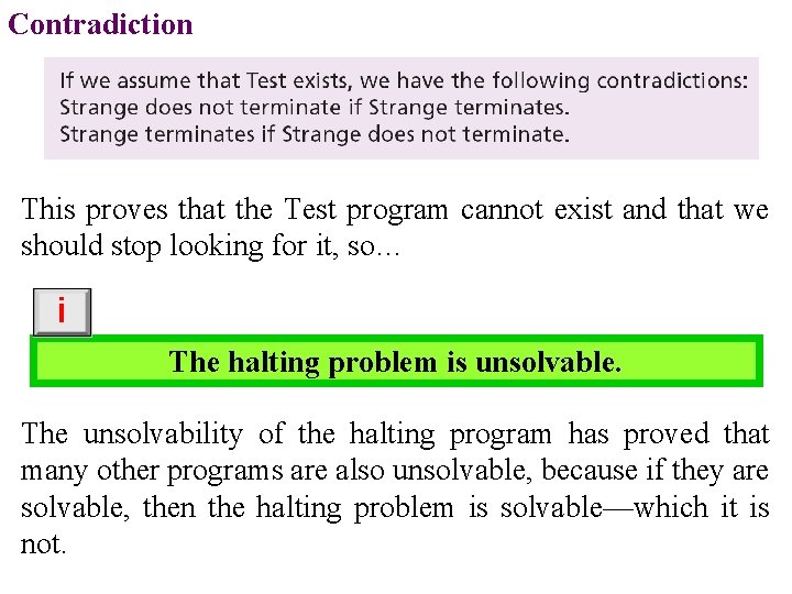
Contradiction This proves that the Test program cannot exist and that we should stop looking for it, so… i The halting problem is unsolvable. The unsolvability of the halting program has proved that many other programs are also unsolvable, because if they are solvable, then the halting problem is solvable—which it is not.

17. 6 COMPLEXITY OF PROBLEMS Now that we have shown that at least one problem is unsolvable by a computer, we’ll touch on this important issue a bit more. In computer science, we can say that, in general, problems can be divided into two categories: solvable problems and unsolvable problems.

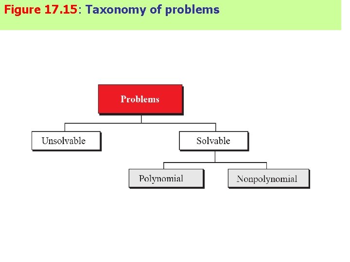
Figure 17. 15: Taxonomy of problems

Solvable problems There are many problems that can be solved by a computer. However, we often want to know how long it takes for the computer to solve that problem. In other words, how complex is the program? The complexity of a program can be measured in several different ways, such as its run time, the memory it needs and so on. One approach is the program’s run time—how long does the program take to run?

Complexity of solvable problems One way to measure the complexity of a solvable problem is to find the number of operations executed by the computer when it runs the program. Big-O notation With the speed of computers today, we are not as concerned with exact numbers as with general orders of magnitude. This simplification of efficiency is known as big-O notation. We present the idea of this notation without delving into its formal definition and calculation. In big-O notation, the number of operations given as a function of the number of inputs. The notation O(n) means a program does n operations for n inputs, while the notation O(n 2) means a program does n 2 operations for n inputs.

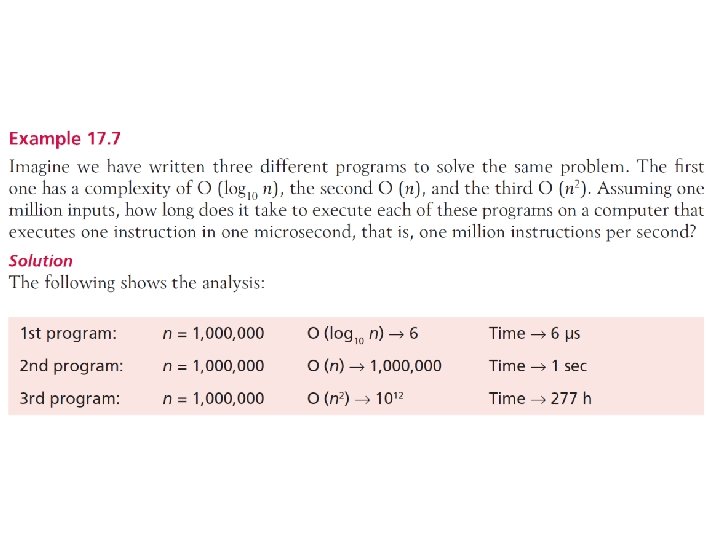
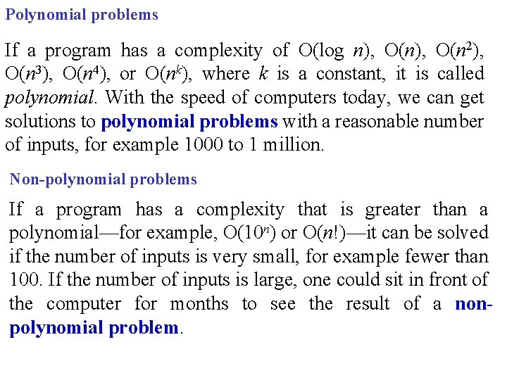
Polynomial problems If a program has a complexity of O(log n), O(n 2), O(n 3), O(n 4), or O(nk), where k is a constant, it is called polynomial. With the speed of computers today, we can get solutions to polynomial problems with a reasonable number of inputs, for example 1000 to 1 million. Non-polynomial problems If a program has a complexity that is greater than a polynomial—for example, O(10 n) or O(n!)—it can be solved if the number of inputs is very small, for example fewer than 100. If the number of inputs is large, one could sit in front of the computer for months to see the result of a nonpolynomial problem.