Objectives of Multiple Regression Establish the linear equation

Objectives of Multiple Regression • Establish the linear equation that best predicts values of a dependent variable Y using more than one explanatory variable from a large set of potential predictors {x 1, x 2, . . . xk}. • Find that subset of all possible predictor variables that explains a significant and appreciable proportion of the variance of Y, trading off adequacy of prediction against the cost of measuring more predictor variables. 1

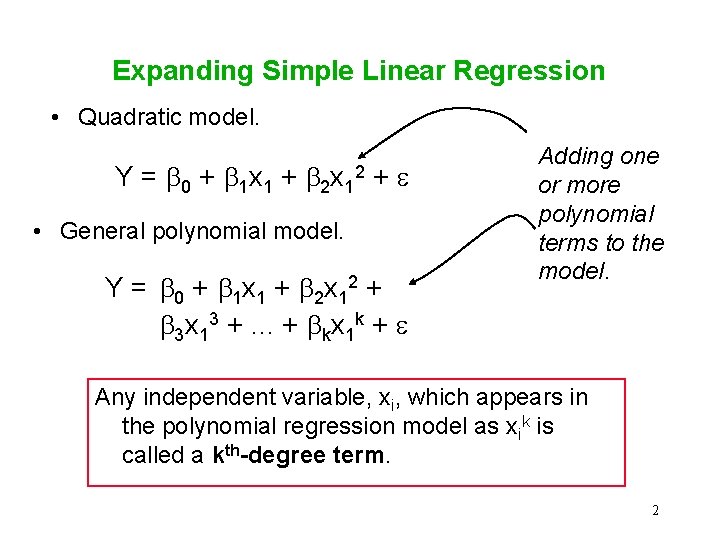
Expanding Simple Linear Regression • Quadratic model. Y = 0 + 1 x 1 + 2 x 1 + e 2 • General polynomial model. Y = 0 + 1 x 1 + 2 x 12 + 3 x 13 +. . . + kx 1 k + e Adding one or more polynomial terms to the model. Any independent variable, xi, which appears in the polynomial regression model as xik is called a kth-degree term. 2

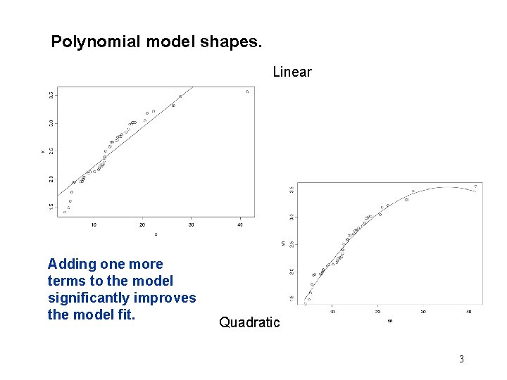
Polynomial model shapes. Linear Adding one more terms to the model significantly improves the model fit. Quadratic 3

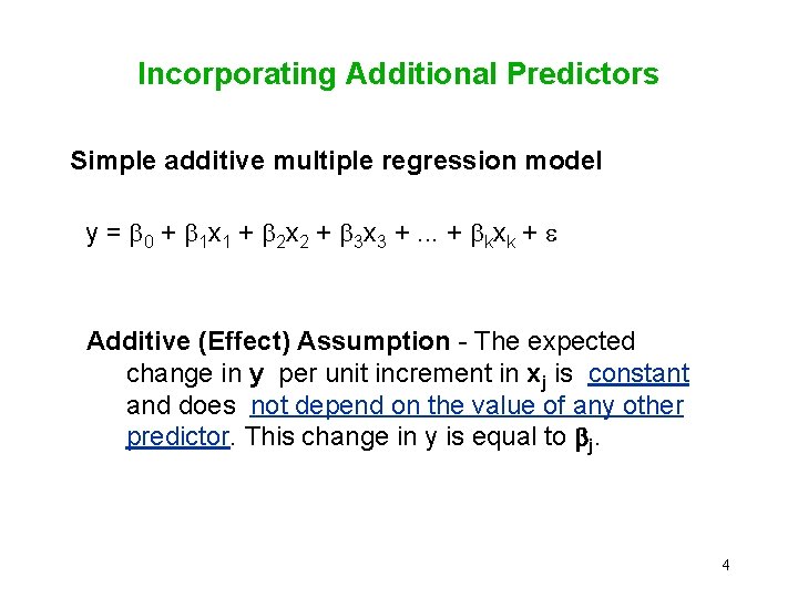
Incorporating Additional Predictors Simple additive multiple regression model y = 0 + 1 x 1 + 2 x 2 + 3 x 3 +. . . + kxk + e Additive (Effect) Assumption - The expected change in y per unit increment in xj is constant and does not depend on the value of any other predictor. This change in y is equal to j. 4

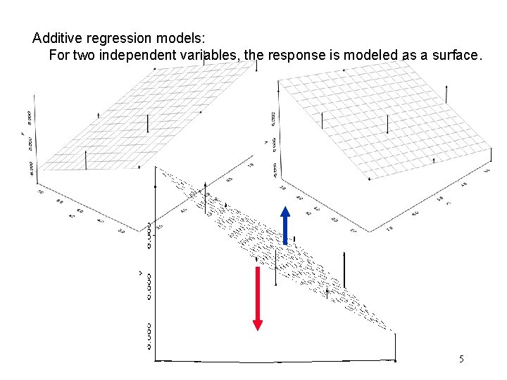
Additive regression models: For two independent variables, the response is modeled as a surface. 5

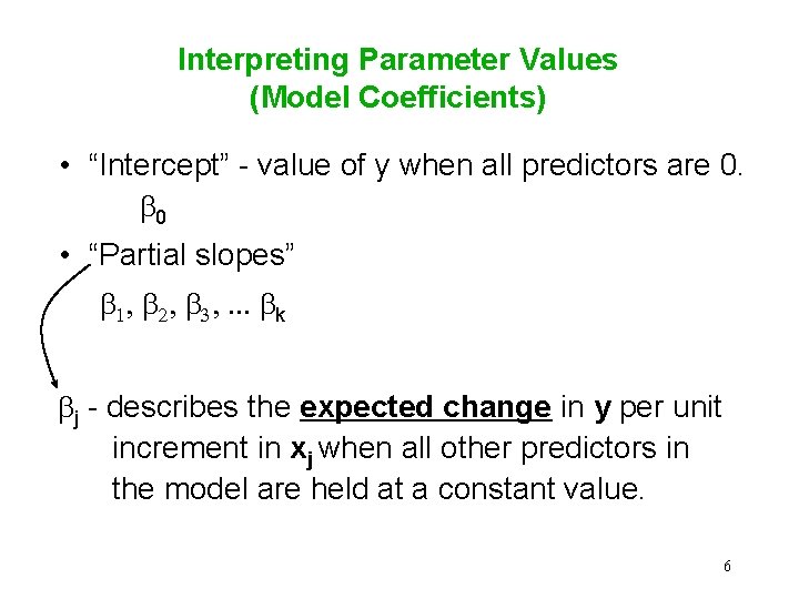
Interpreting Parameter Values (Model Coefficients) • “Intercept” - value of y when all predictors are 0. 0 • “Partial slopes” 1, 2, 3, . . . k j - describes the expected change in y per unit increment in xj when all other predictors in the model are held at a constant value. 6

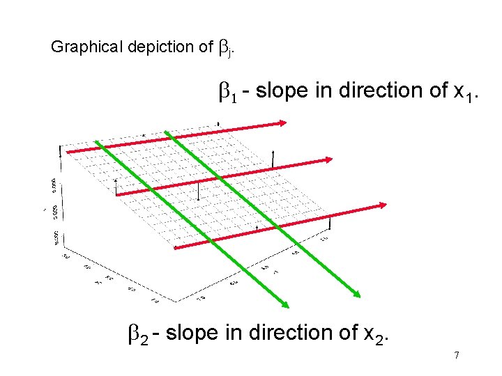
Graphical depiction of j. 1 - slope in direction of x 1. 2 - slope in direction of x 2. 7

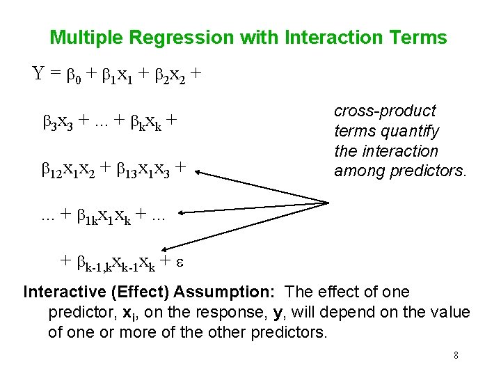
Multiple Regression with Interaction Terms Y = 0 + 1 x 1 + 2 x 2 + 3 x 3 +. . . + kxk + 12 x 1 x 2 + 13 x 1 x 3 + cross-product terms quantify the interaction among predictors. . + 1 kx 1 xk +. . . + k-1, kxk-1 xk + e Interactive (Effect) Assumption: The effect of one predictor, xi, on the response, y, will depend on the value of one or more of the other predictors. 8

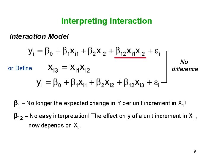
Interpreting Interaction Model or Define: No difference 1 – No longer the expected change in Y per unit increment in X 1! 12 – No easy interpretation! The effect on y of a unit increment in X 1, now depends on X 2. 9

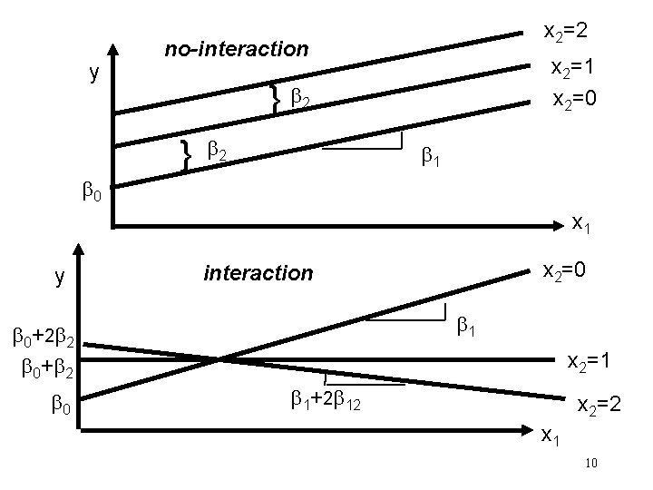
y x 2=2 no-interaction } } x 2=1 x 2=0 2 2 1 0 x 1 y 1 0+ 2 2 0+ 2 0 x 2=0 interaction x 2=1 1+2 12 x 2=2 x 1 10

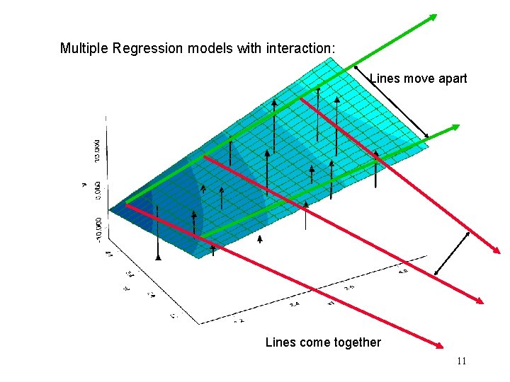
Multiple Regression models with interaction: Lines move apart Lines come together 11

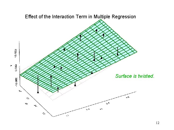
Effect of the Interaction Term in Multiple Regression Surface is twisted. 12

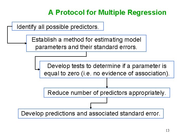
A Protocol for Multiple Regression Identify all possible predictors. Establish a method for estimating model parameters and their standard errors. Develop tests to determine if a parameter is equal to zero (i. e. no evidence of association). Reduce number of predictors appropriately. Develop predictions and associated standard error. 13

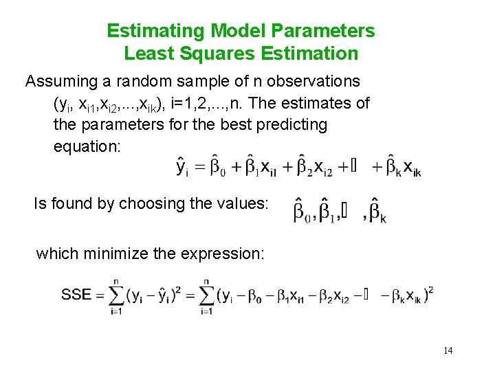
Estimating Model Parameters Least Squares Estimation Assuming a random sample of n observations (yi, xi 1, xi 2, . . . , xik), i=1, 2, . . . , n. The estimates of the parameters for the best predicting equation: Is found by choosing the values: which minimize the expression: 14

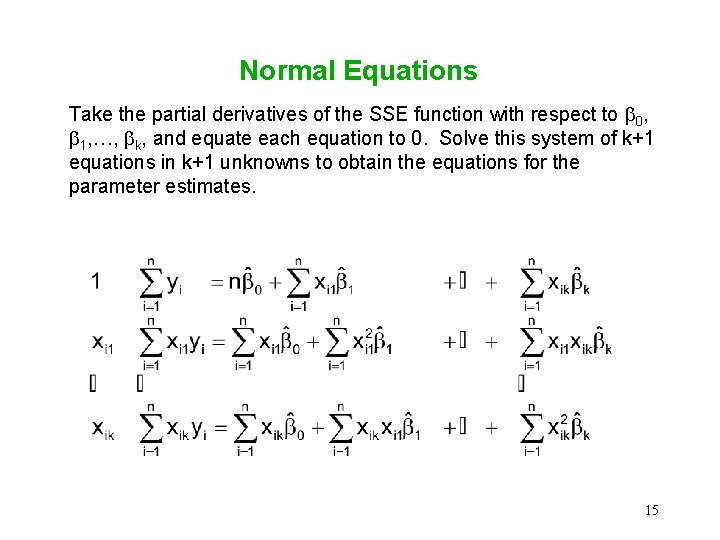
Normal Equations Take the partial derivatives of the SSE function with respect to 0, 1, …, k, and equate each equation to 0. Solve this system of k+1 equations in k+1 unknowns to obtain the equations for the parameter estimates. 15

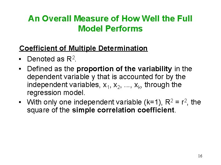
An Overall Measure of How Well the Full Model Performs Coefficient of Multiple Determination • Denoted as R 2. • Defined as the proportion of the variability in the dependent variable y that is accounted for by the independent variables, x 1, x 2, . . . , xk, through the regression model. • With only one independent variable (k=1), R 2 = r 2, the square of the simple correlation coefficient. 16

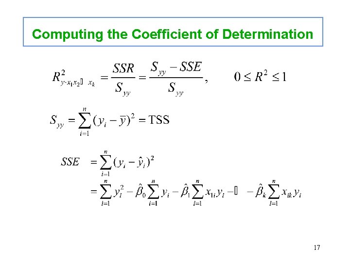
Computing the Coefficient of Determination 17

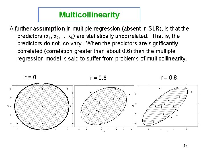
Multicollinearity A further assumption in multiple regression (absent in SLR), is that the predictors (x 1, x 2, . . . xk) are statistically uncorrelated. That is, the predictors do not co-vary. When the predictors are significantly correlated (correlation greater than about 0. 6) then the multiple regression model is said to suffer from problems of multicollinearity. r=0 r = 0. 6 r = 0. 8 18

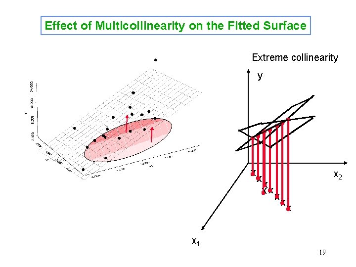
Effect of Multicollinearity on the Fitted Surface Extreme collinearity y x xx x 2 x x 1 19

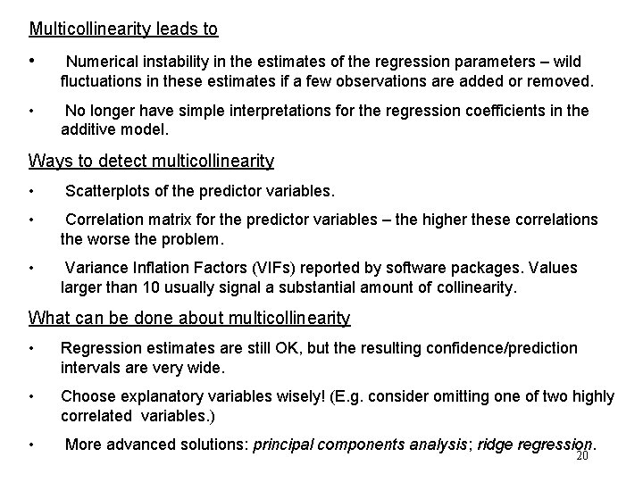
Multicollinearity leads to • Numerical instability in the estimates of the regression parameters – wild fluctuations in these estimates if a few observations are added or removed. • No longer have simple interpretations for the regression coefficients in the additive model. Ways to detect multicollinearity • Scatterplots of the predictor variables. • Correlation matrix for the predictor variables – the higher these correlations the worse the problem. • Variance Inflation Factors (VIFs) reported by software packages. Values larger than 10 usually signal a substantial amount of collinearity. What can be done about multicollinearity • Regression estimates are still OK, but the resulting confidence/prediction intervals are very wide. • Choose explanatory variables wisely! (E. g. consider omitting one of two highly correlated variables. ) • More advanced solutions: principal components analysis; ridge regression. 20

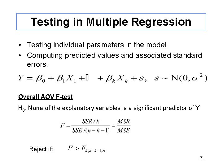
Testing in Multiple Regression • Testing individual parameters in the model. • Computing predicted values and associated standard errors. Overall AOV F-test H 0: None of the explanatory variables is a significant predictor of Y Reject if: 21

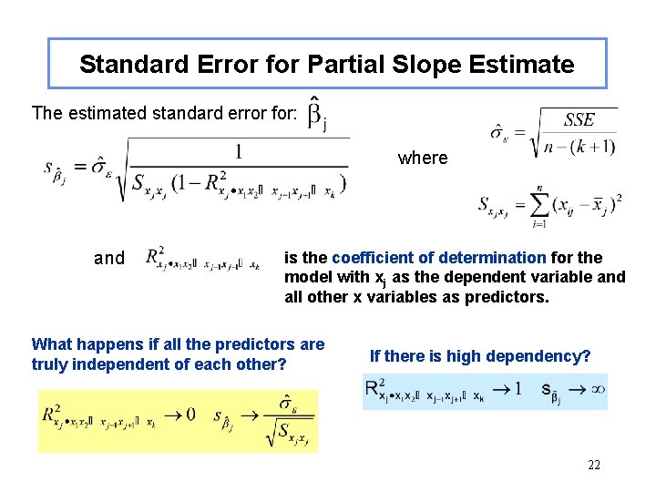
Standard Error for Partial Slope Estimate The estimated standard error for: where and is the coefficient of determination for the model with xj as the dependent variable and all other x variables as predictors. What happens if all the predictors are truly independent of each other? If there is high dependency? 22

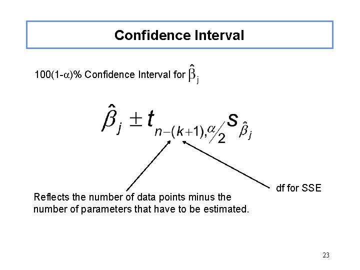
Confidence Interval 100(1 -a)% Confidence Interval for Reflects the number of data points minus the number of parameters that have to be estimated. df for SSE 23

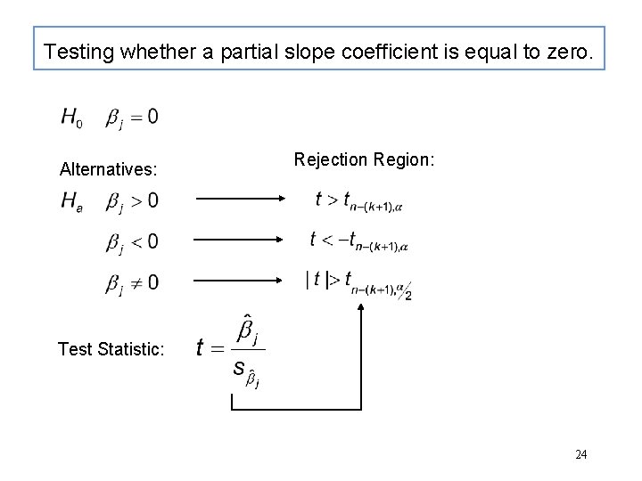
Testing whether a partial slope coefficient is equal to zero. Alternatives: Rejection Region: Test Statistic: 24

Predicting Y • We use the least squares fitted value, , as our predictor of a single value of y at a particular value of the explanatory variables (x 1, x 2, . . . , xk). • The corresponding interval about the predicted value of y is called a prediction interval. • The least squares fitted value also provides the best predictor of E(y), the mean value of y, at a particular value of (x 1, x 2, . . . , xk). The corresponding interval for the mean prediction is called a confidence interval. • Formulas for these intervals are much more complicated than in the case of SLR; they cannot be calculated by hand (see the book). 25

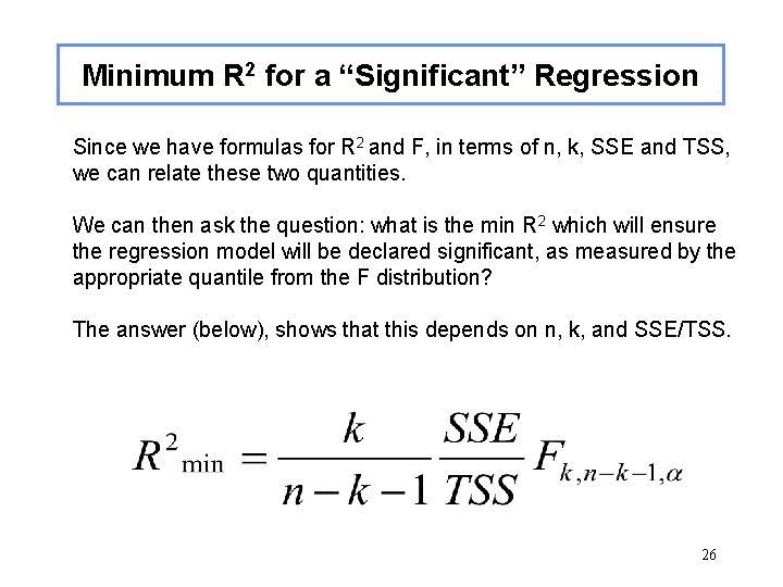
Minimum R 2 for a “Significant” Regression Since we have formulas for R 2 and F, in terms of n, k, SSE and TSS, we can relate these two quantities. We can then ask the question: what is the min R 2 which will ensure the regression model will be declared significant, as measured by the appropriate quantile from the F distribution? The answer (below), shows that this depends on n, k, and SSE/TSS. 26

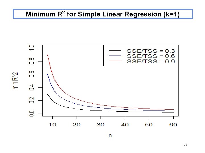
Minimum R 2 for Simple Linear Regression (k=1) 27