Objectives of Image Coding Representation of an image
Objectives of Image Coding • Representation of an image with acceptable quality, using as small a number of bits as possible Applications: • Reduction of channel bandwidth for image transmission • Reduction of required storage
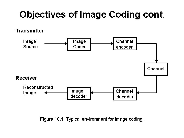
Objectives of Image Coding cont. Transmitter Image Source Image Coder Channel encoder Channel Receiver Reconstructed Image decoder Channel decoder Figure 10. 1 Typical environment for image coding.
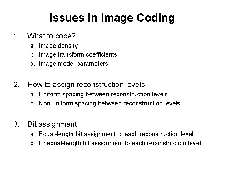
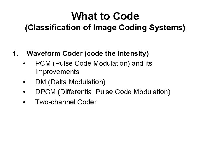
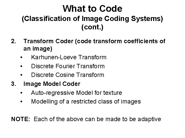
Issues in Image Coding 1. What to code? a. Image density b. Image transform coefficients c. Image model parameters 2. How to assign reconstruction levels a. Uniform spacing between reconstruction levels b. Non-uniform spacing between reconstruction levels 3. Bit assignment a. Equal-length bit assignment to each reconstruction level b. Unequal-length bit assignment to each reconstruction level
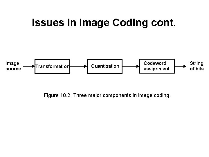
Issues in Image Coding cont. Image source Transformation Quantization Codeword assignment Figure 10. 2 Three major components in image coding. String of bits
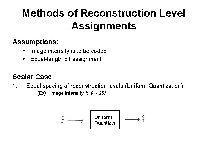
Methods of Reconstruction Level Assignments Assumptions: • Image intensity is to be coded • Equal-length bit assignment Scalar Case 1. Equal spacing of reconstruction levels (Uniform Quantization) (Ex): Image intensity f: 0 ~ 255 Uniform Quantizer
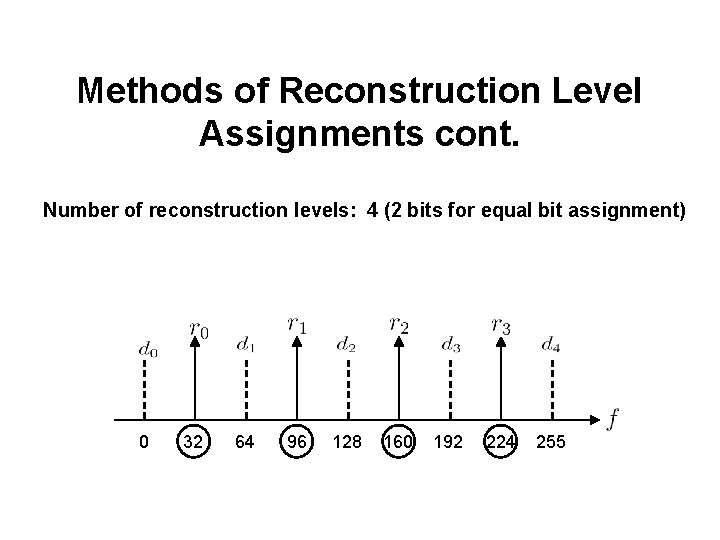
Methods of Reconstruction Level Assignments cont. Number of reconstruction levels: 4 (2 bits for equal bit assignment) 0 32 64 96 128 160 192 224 255
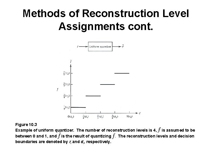
Methods of Reconstruction Level Assignments cont. Figure 10. 3 Example of uniform quantizer. The number of reconstruction levels is 4, is assumed to be between 0 and 1, and is the result of quantizing. The reconstruction levels and decision boundaries are denoted by ri and di, respectively.
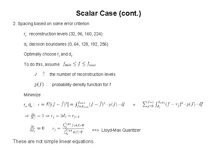
Scalar Case (cont. ) 2. Spacing based on some error criterion ri: reconstruction levels (32, 96, 160, 224) di: decision boundaries (0, 64, 128, 192, 256) Optimally choose ri and di. To do this, assume J the number of reconstruction levels : probability density function for f Minimize ri, di, : = ==> Lloyd-Max Quantizer These are not simple linear equations.
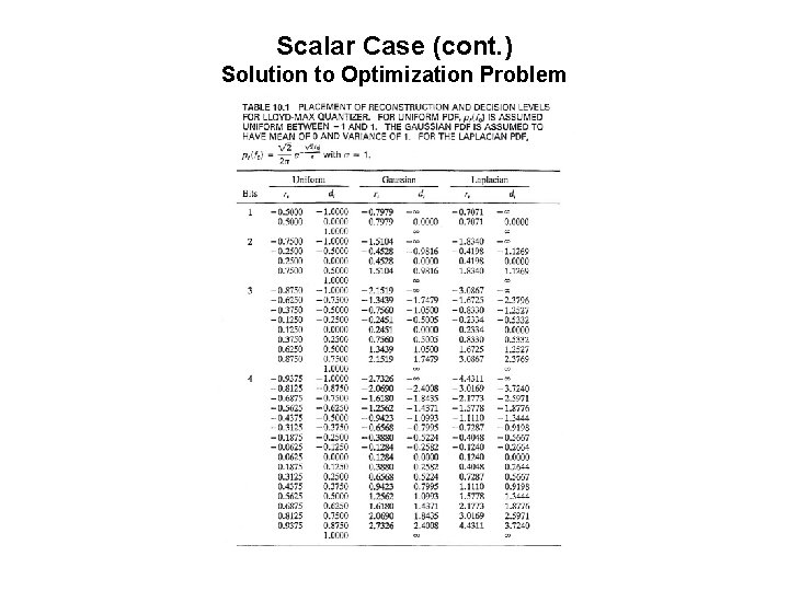
Scalar Case (cont. ) Solution to Optimization Problem
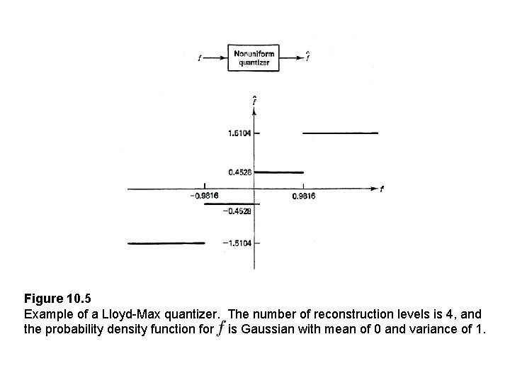
Figure 10. 5 Example of a Lloyd-Max quantizer. The number of reconstruction levels is 4, and the probability density function for is Gaussian with mean of 0 and variance of 1.
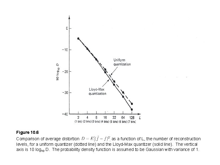
Figure 10. 6 Comparison of average distortion as a function of L, the number of reconstruction levels, for a uniform quantizer (dotted line) and the Lloyd-Max quantizer (solid line). The vertical axis is 10 log 10 D. The probability density function is assumed to be Gaussian with variance of 1.
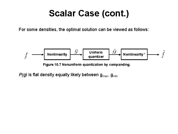
Scalar Case (cont. ) For some densities, the optimal solution can be viewed as follows: Nonlinearity Uniform quantizer Nonlinearity-1 Figure 10. 7 Nonuniform quantization by companding. P(g) is flat density equally likely between gmax, gmin
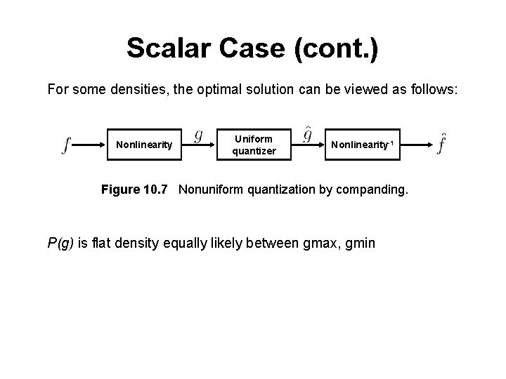
Scalar Case (cont. ) For some densities, the optimal solution can be viewed as follows: Nonlinearity Uniform quantizer Nonlinearity-1 Figure 10. 7 Nonuniform quantization by companding. P(g) is flat density equally likely between gmax, gmin
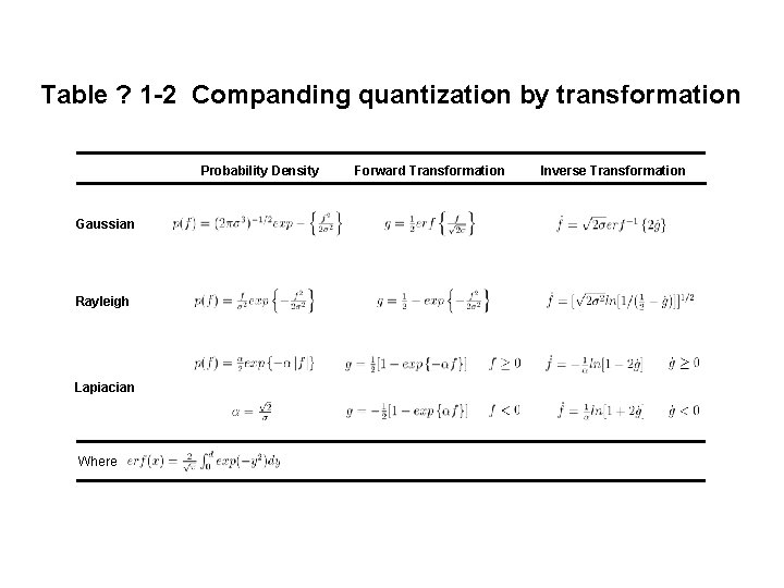
Table ? 1 -2 Companding quantization by transformation Probability Density Gaussian Rayleigh Lapiacian Where Forward Transformation Inverse Transformation
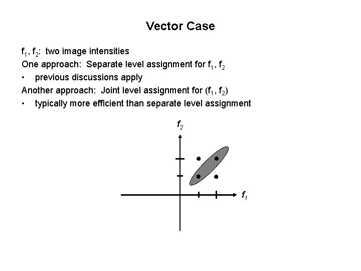
Vector Case f 1, f 2: two image intensities One approach: Separate level assignment for f 1, f 2 • previous discussions apply Another approach: Joint level assignment for (f 1, f 2) • typically more efficient than separate level assignment f 2 f 1
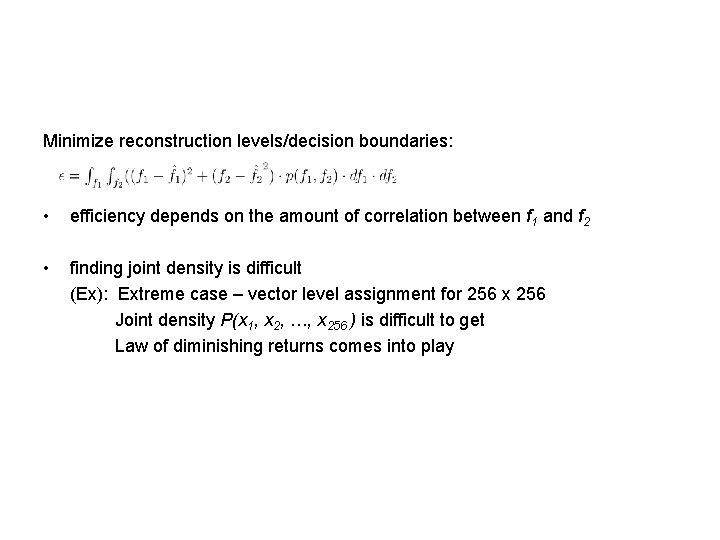
Minimize reconstruction levels/decision boundaries: • efficiency depends on the amount of correlation between f 1 and f 2 • finding joint density is difficult (Ex): Extreme case – vector level assignment for 256 x 256 Joint density P(x 1, x 2, …, x 256 ) is difficult to get Law of diminishing returns comes into play
Codeword Design: Bit Allocation • After quantization, need to assign binray codeword to each quantization symbol. • Options: – Uniform: equal number of bits to each symbol inefficient – Non-uniform: short codewords to more probable symbols, and longer codewords for less probable ones. • For non-uniform, code has to be uniquely decodable: – Example: L = 4, r 1 0, r 2 1, r 3 10, r 4 11 – Suppose we receive 100. – Can decode it two ways: either r 3 r 1 or r 2 r 1 r 1. – Not uniquely decodable. – One codeword is a prefix of another one. • Use Prefix codes instead to achieve unique decodability.
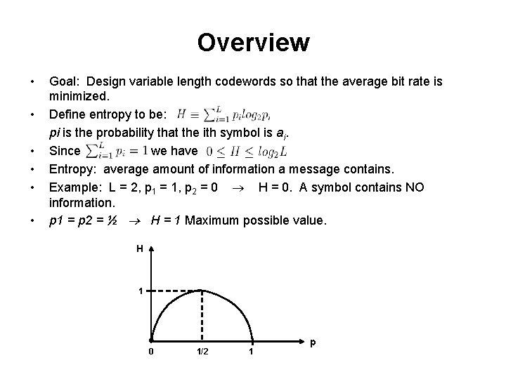
Overview • • • Goal: Design variable length codewords so that the average bit rate is minimized. Define entropy to be: pi is the probability that the ith symbol is ai. Since we have Entropy: average amount of information a message contains. Example: L = 2, p 1 = 1, p 2 = 0 H = 0. A symbol contains NO information. p 1 = p 2 = ½ H = 1 Maximum possible value. H 1 0 1/2 1 p
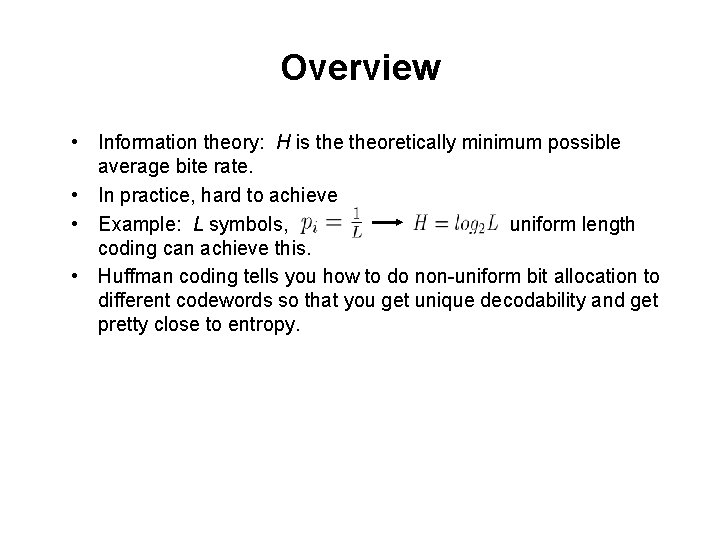
Overview • Information theory: H is theoretically minimum possible average bite rate. • In practice, hard to achieve • Example: L symbols, uniform length coding can achieve this. • Huffman coding tells you how to do non-uniform bit allocation to different codewords so that you get unique decodability and get pretty close to entropy.
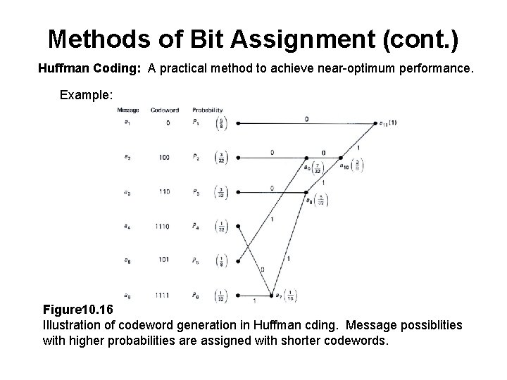
Methods of Bit Assignment (cont. ) Huffman Coding: A practical method to achieve near-optimum performance. Example: Figure 10. 16 Illustration of codeword generation in Huffman cding. Message possiblities with higher probabilities are assigned with shorter codewords.
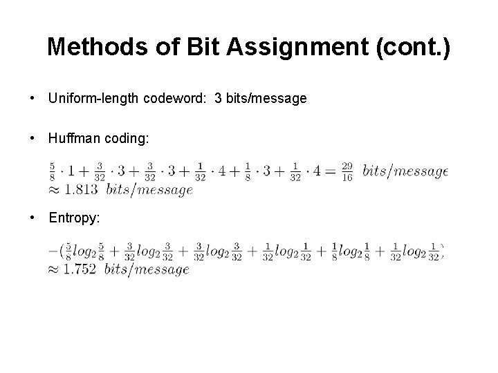
Methods of Bit Assignment (cont. ) • Uniform-length codeword: 3 bits/message • Huffman coding: • Entropy:
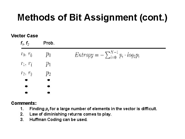
Methods of Bit Assignment (cont. ) Vector Case f 1 , f 2 Prob. Comments: 1. 2. 3. Finding pi for a large number of elements in the vector is difficult. Law of diminishing returns comes to play. Huffman Coding can be used.
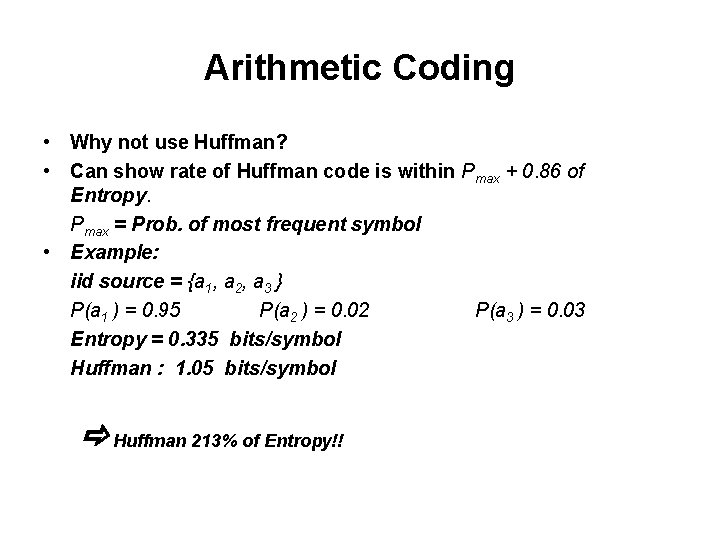
Arithmetic Coding • Why not use Huffman? • Can show rate of Huffman code is within Pmax + 0. 86 of Entropy. Pmax = Prob. of most frequent symbol • Example: iid source = {a 1, a 2, a 3 } P(a 1 ) = 0. 95 P(a 2 ) = 0. 02 P(a 3 ) = 0. 03 Entropy = 0. 335 bits/symbol Huffman : 1. 05 bits/symbol Huffman 213% of Entropy!!
Mechanics fo Arithmetic Coding • Two Steps: 1. Generate a tag 2. Assign a binary code to the tag • Tag Generation: A sequence of symbols from an alphabet source with a given Pdf results in a unique sub-interval in [0, 1].
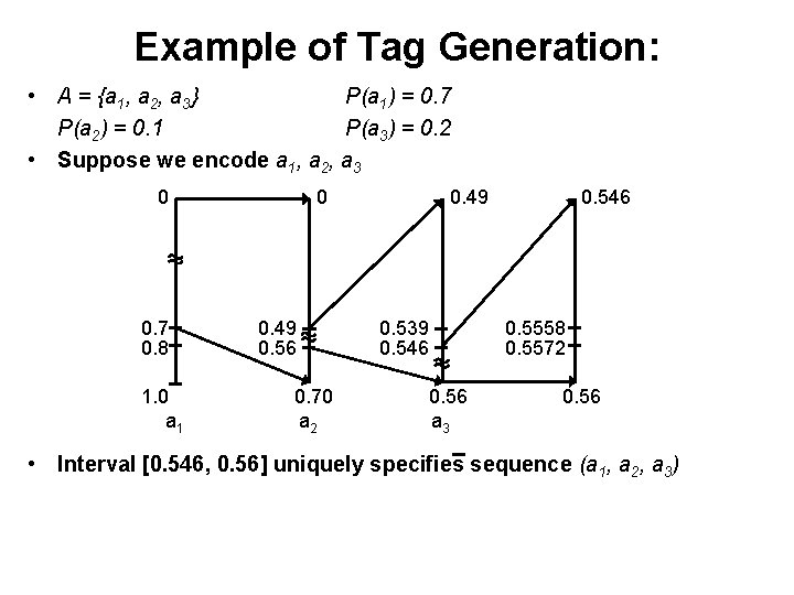
Example of Tag Generation: • A = {a 1, a 2, a 3} P(a 1) = 0. 7 P(a 2) = 0. 1 P(a 3) = 0. 2 • Suppose we encode a 1, a 2, a 3 0 0. 7 0. 8 1. 0 a 1 0 0. 49 0. 56 0. 70 a 2 0. 49 0. 539 0. 546 0. 56 a 3 0. 546 0. 5558 0. 5572 0. 56 • Interval [0. 546, 0. 56] uniquely specifies sequence (a 1, a 2, a 3)
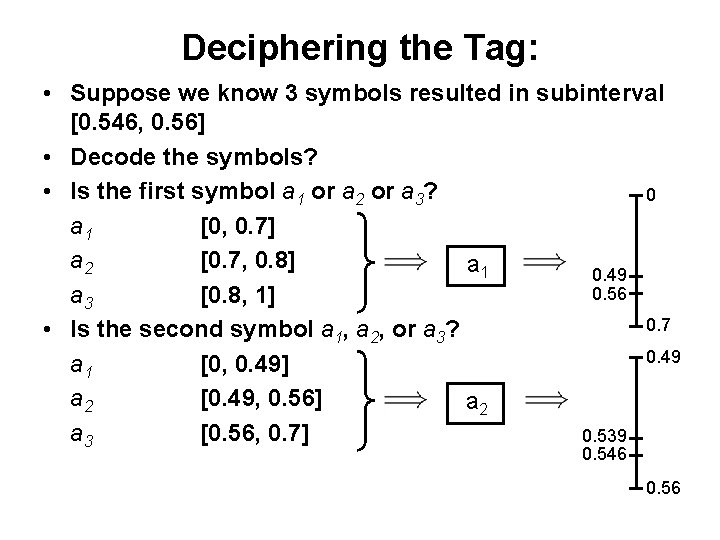
Deciphering the Tag: • Suppose we know 3 symbols resulted in subinterval [0. 546, 0. 56] • Decode the symbols? • Is the first symbol a 1 or a 2 or a 3? 0 a 1 [0, 0. 7] a 2 [0. 7, 0. 8] a 1 0. 49 0. 56 a 3 [0. 8, 1] 0. 7 • Is the second symbol a 1, a 2, or a 3? 0. 49 a 1 [0, 0. 49] a 2 [0. 49, 0. 56] a 2 a 3 [0. 56, 0. 7] 0. 539 0. 546 0. 56
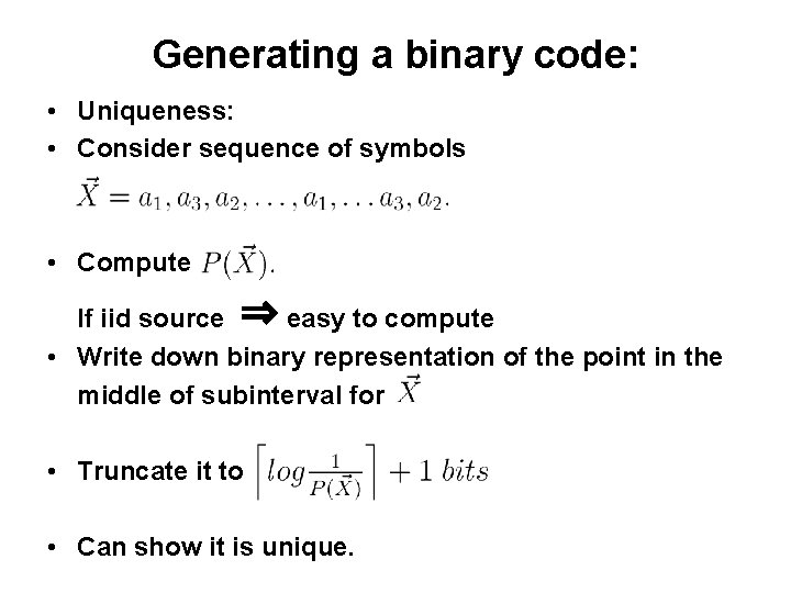
Generating a binary code: • Uniqueness: • Consider sequence of symbols • Compute If iid source ⇒ easy to compute • Write down binary representation of the point in the middle of subinterval for • Truncate it to • Can show it is unique.
![Example Generating a binary code: • Consider subinterval [0. 546, 0. 56] • Midpoint: Example Generating a binary code: • Consider subinterval [0. 546, 0. 56] • Midpoint:](http://slidetodoc.com/presentation_image_h/260d87091c9951675be7fa637bce8be1/image-28.jpg)
Example Generating a binary code: • Consider subinterval [0. 546, 0. 56] • Midpoint: 0. 553 • • # of bits = • Binary Representation of 0. 553 • Truncate to 8 bits 10001101 ⇒ Binary Representation:
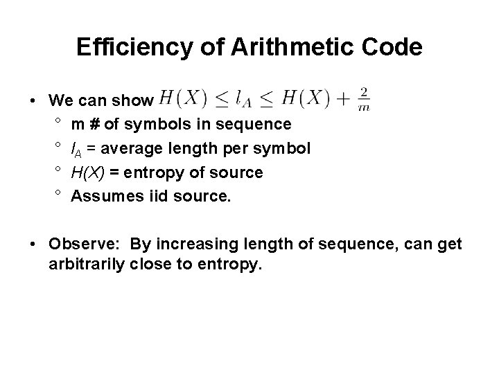
Efficiency of Arithmetic Code • We can show ° m # of symbols in sequence ° l. A = average length per symbol ° H(X) = entropy of source ° Assumes iid source. • Observe: By increasing length of sequence, can get arbitrarily close to entropy.
Dictionary Techniques • Huffman and arithmetic coding assumed i. i. d. sources • Most sources are correlated • Main idea: 1. Build a list of commonly occurring patterns 2. Transmit index in the list. • Exploits fact that certain patterns recur frequently. • Consider 2 cases: 1. Static Dictionary 2. Dynamic Dictionary
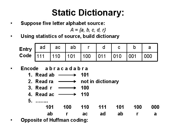
Static Dictionary: • • Suppose five letter alphabet source: A = {a, b, c, d, r} Using statistics of source, build dictionary ad Entry Code 111 • • ac ab r d c b a 110 101 100 011 010 001 000 Encode a b r a c a d a b r a 1. Read ab 101 2. Read ra not in dictionary 3. Read r 100 4. Read ac 110 5. ……. . 101 100 111 101 ab r ac ad ab Opposite of Huffman coding: 100 r 000 a
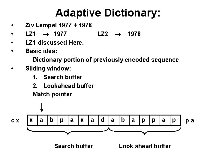
Adaptive Dictionary: • • • cx Ziv Lempel 1977 + 1978 LZ 1 1977 LZ 2 1978 LZ 1 discussed Here. Basic idea: Dictionary portion of previously encoded sequence Sliding window: 1. Search buffer 2. Lookahead buffer Match pointer x a b p a x a Search buffer d a b a p p a Look ahead buffer p pa
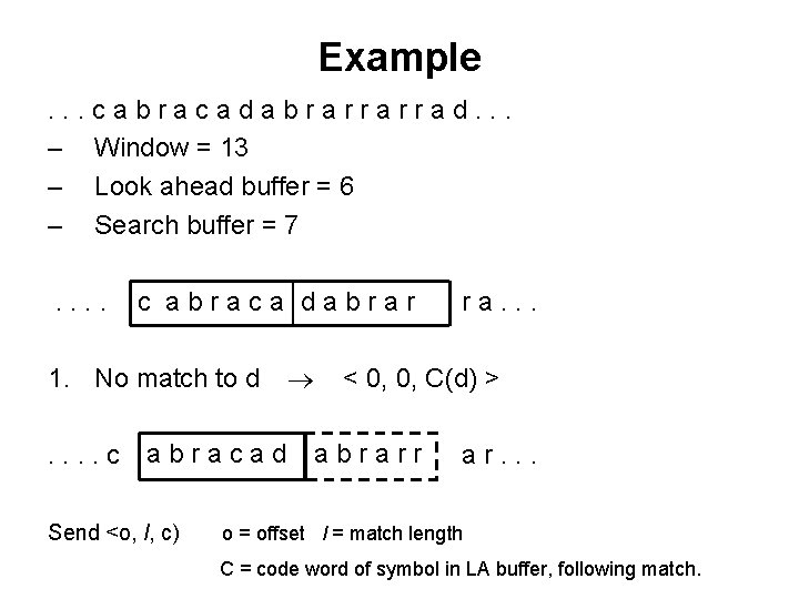
Example. . . cabracadabrarrarrad. . . – Window = 13 – Look ahead buffer = 6 – Search buffer = 7. . c abraca dabrar 1. No match to d. . c abracad Send <o, l, c) ra. . . < 0, 0, C(d) > abrarr ar. . . o = offset l = match length C = code word of symbol in LA buffer, following match.
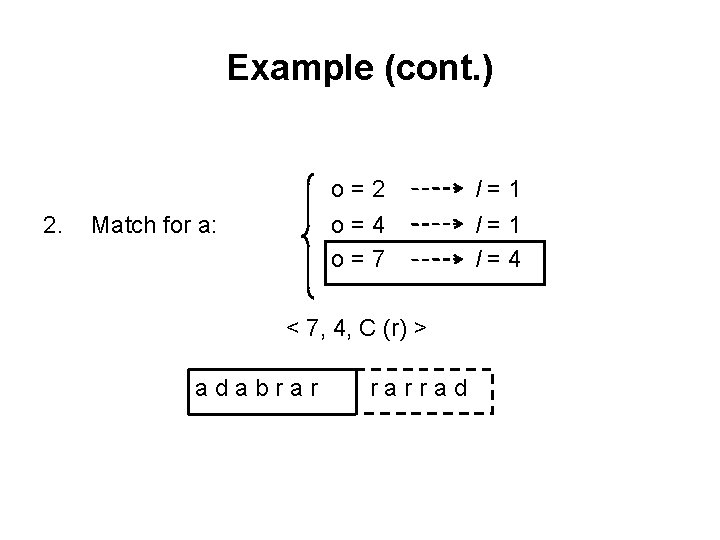
Example (cont. ) 2. o=2 o=4 o=7 Match for a: < 7, 4, C (r) > adabrar rarrad l=1 l=4
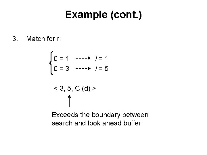
Example (cont. ) 3. Match for r: 0=1 0=3 l=1 l=5 < 3, 5, C (d) > Exceeds the boundary between search and look ahead buffer
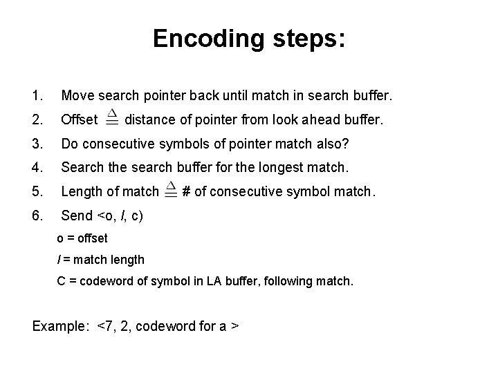
Encoding steps: 1. Move search pointer back until match in search buffer. 2. Offset 3. Do consecutive symbols of pointer match also? 4. Search the search buffer for the longest match. 5. Length of match 6. Send <o, l, c) distance of pointer from look ahead buffer. # of consecutive symbol match. o = offset l = match length C = codeword of symbol in LA buffer, following match. Example: <7, 2, codeword for a >
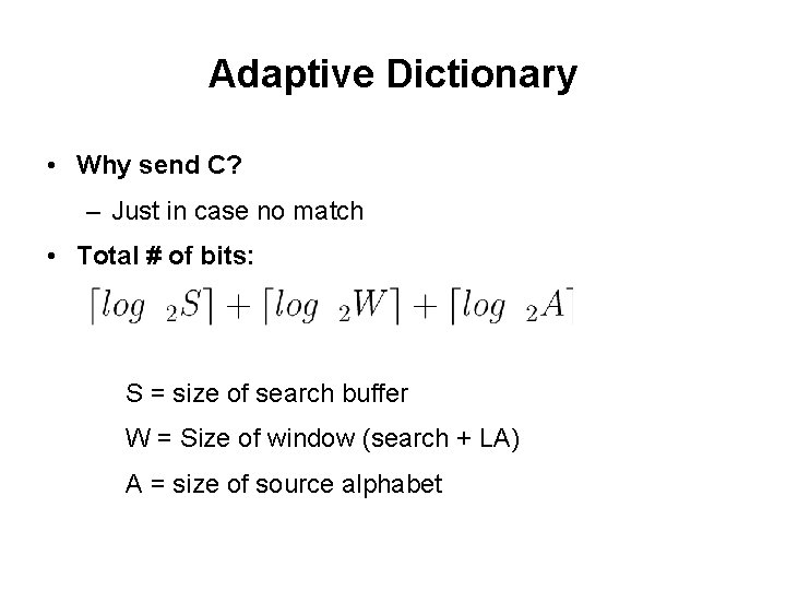
Adaptive Dictionary • Why send C? – Just in case no match • Total # of bits: S = size of search buffer W = Size of window (search + LA) A = size of source alphabet
What to Code (Classification of Image Coding Systems) 1. Waveform Coder (code the intensity) • PCM (Pulse Code Modulation) and its improvements • DM (Delta Modulation) • DPCM (Differential Pulse Code Modulation) • Two-channel Coder
What to Code (Classification of Image Coding Systems) (cont. ) 2. Transform Coder (code transform coefficients of an image) • Karhunen-Loeve Transform • Discrete Fourier Transform • Discrete Cosine Transform 3. Image Model Coder • Auto-regressive Model for texture • Modelling of a restricted class of images NOTE: Each of the above can be made to be adaptive
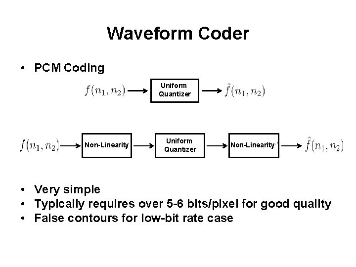
Waveform Coder • PCM Coding Uniform Quantizer Non-Linearity-1 • Very simple • Typically requires over 5 -6 bits/pixel for good quality • False contours for low-bit rate case
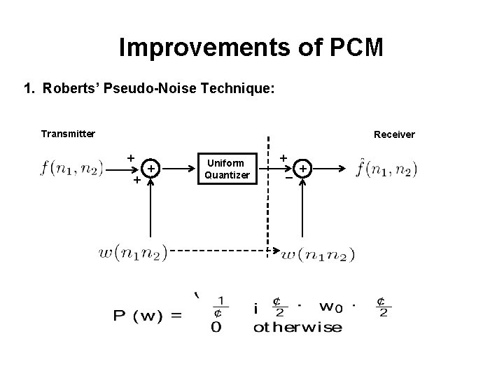
Improvements of PCM 1. Roberts’ Pseudo-Noise Technique: Transmitter Receiver + + + Uniform Quantizer + _ +
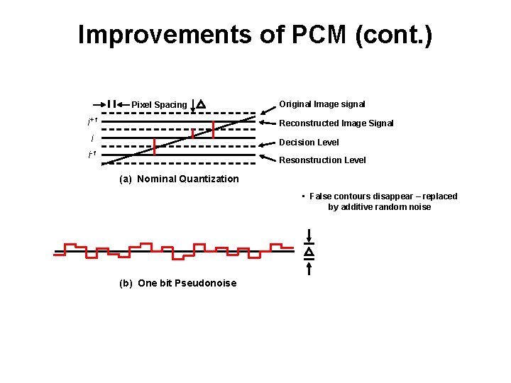
Improvements of PCM (cont. ) Pixel Spacing i+1 Original Image signal Reconstructed Image Signal i Decision Level i-1 Resonstruction Level (a) Nominal Quantization • False contours disappear – replaced by additive random noise (b) One bit Pseudonoise
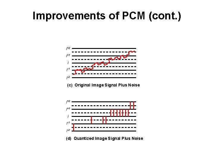
Improvements of PCM (cont. ) i+2 i+1 i i-1 i-2 (c) Original Image Signal Plus Noise i+2 i+1 i i-1 i-2 (d) Quantized Image Signal Plus Noise
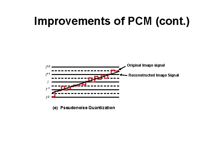
Improvements of PCM (cont. ) Original Image signal i+2 i+1 Reconstructed Image Signal i i-1 i-2 (e) Pseudonoise Quantization
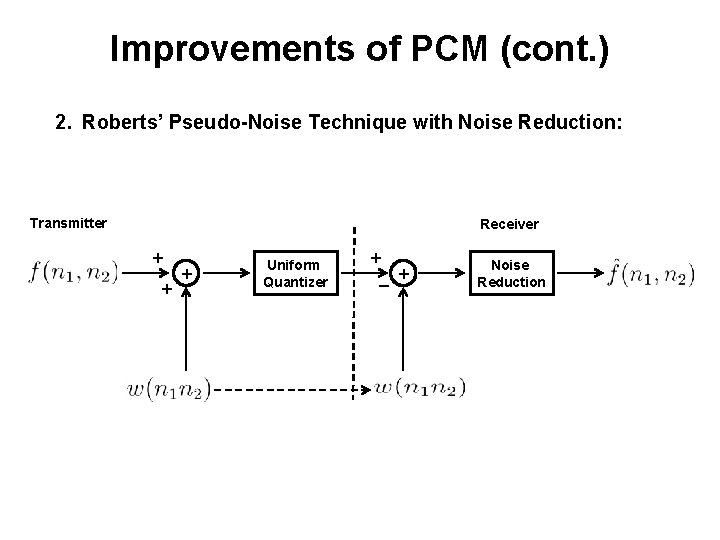
Improvements of PCM (cont. ) 2. Roberts’ Pseudo-Noise Technique with Noise Reduction: Transmitter Receiver + + + Uniform Quantizer + _ + Noise Reduction
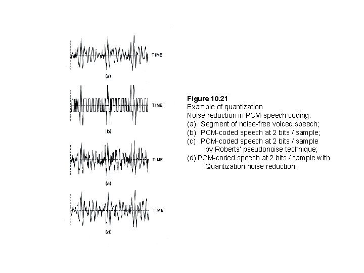
Figure 10. 21 Example of quantization Noise reduction in PCM speech coding. (a) Segment of noise-free voiced speech; (b) PCM-coded speech at 2 bits / sample; (c) PCM-coded speech at 2 bits / sample by Roberts’ pseudonoise technique; (d) PCM-coded speech at 2 bits / sample with Quantization noise reduction.
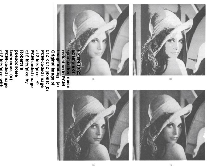
Figure 10. 22 Example of quantization noise reduction in PCM image coding. (a) Original image of 512 x 512 pixels; (b) PCM-coded image at 2 bits/pixel; © PCM-coded image at 2 bits/pixel by Roberts’s pseudonoise technique; (d) PCM-coded image
Delta Modulation (DM) Transmitter + _ + 1 bit quantization +
Delta Modulation (DM) (cont. ) Receiver +
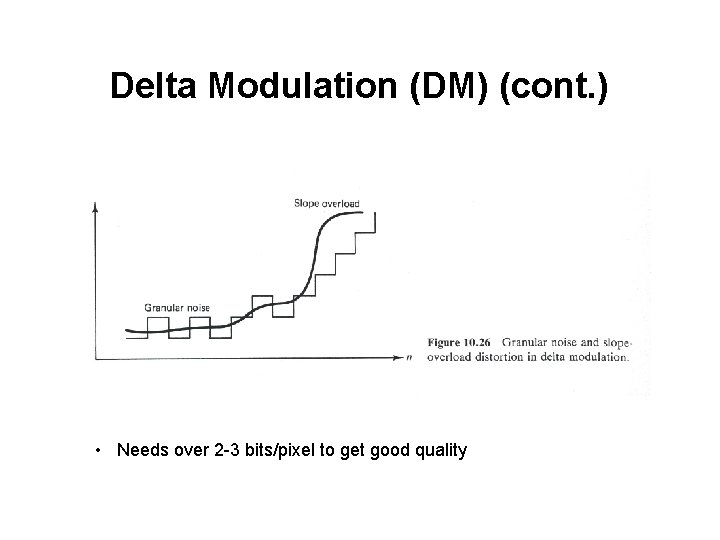
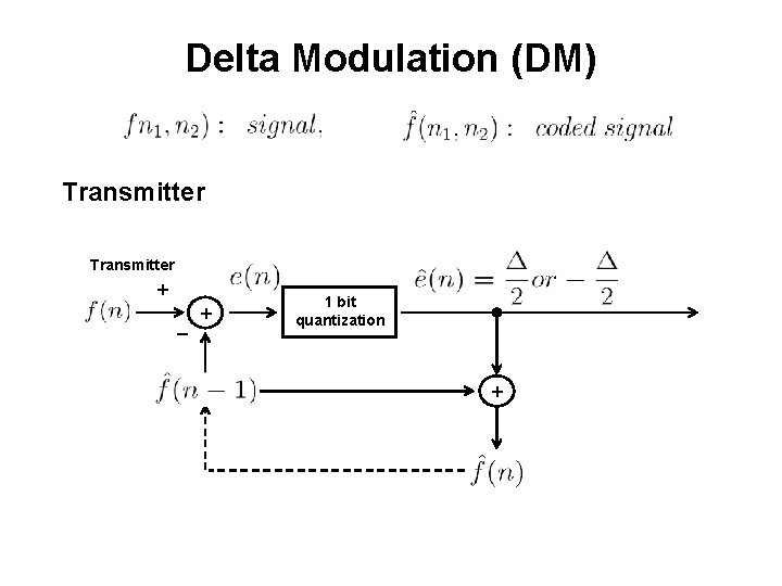
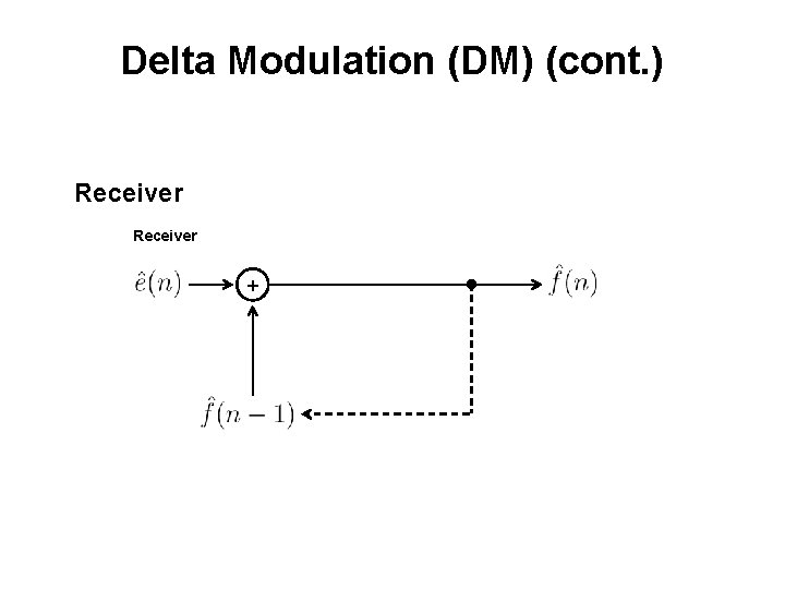
Delta Modulation (DM) (cont. ) • Needs over 2 -3 bits/pixel to get good quality
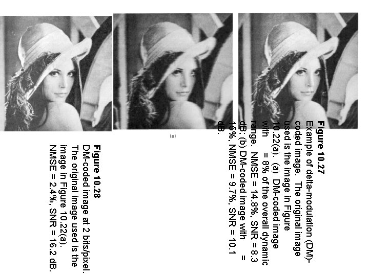
Figure 10. 27 Example of delta-modulation (DM)coded image. The original image used is the image in Figure 10. 22(a). (a) DM-coded image with = 8% of the overall dynamic range. NMSE = 14. 8%, SNR = 8. 3 d. B; (b) DM-coded image with = 15%, NMSE = 9. 7%, SNR = 10. 1 d. B. Figure 10. 28 DM-coded image at 2 bits/pixel. The original image used is the image in Figure 10. 22(a). NMSE = 2. 4%, SNR = 16. 2 d. B.
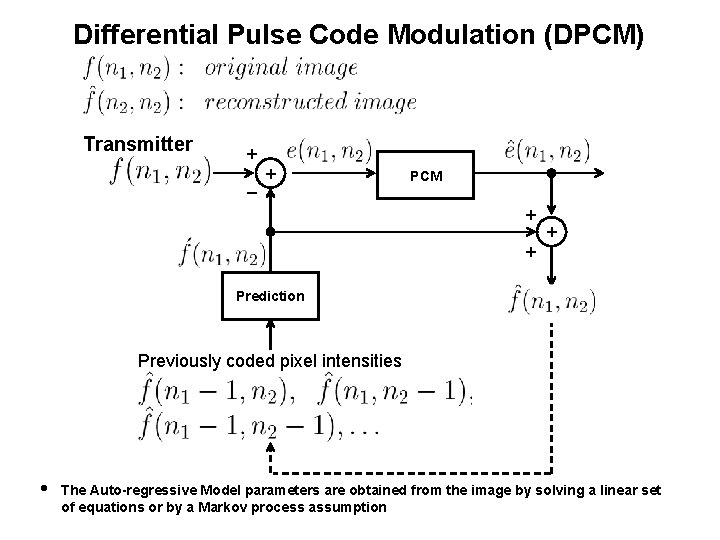
Differential Pulse Code Modulation (DPCM) Transmitter + _ + PCM + + + Prediction Previously coded pixel intensities The Auto-regressive Model parameters are obtained from the image by solving a linear set of equations or by a Markov process assumption
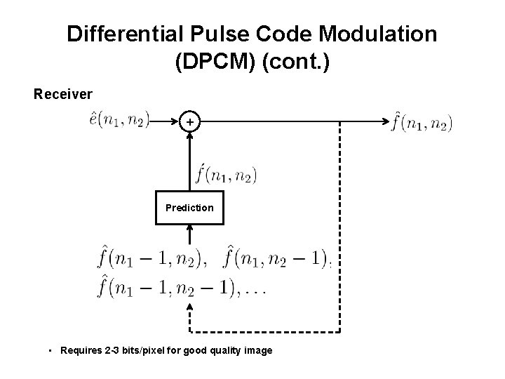
Differential Pulse Code Modulation (DPCM) (cont. ) Receiver + Prediction • Requires 2 -3 bits/pixel for good quality image
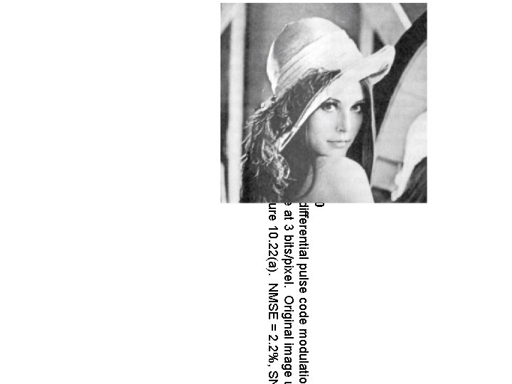
Figure 10. 30 Example of differential pulse code modulatio coded image at 3 bits/pixel. Original image u image in Figure 10. 22(a). NMSE = 2. 2%, SN
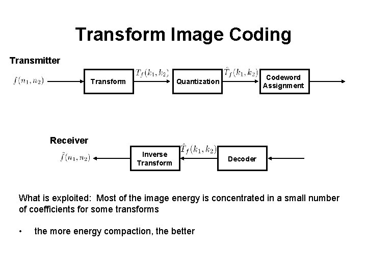
Transform Image Coding Transmitter Transform Codeword Assignment Quantization Receiver Inverse Transform Decoder What is exploited: Most of the image energy is concentrated in a small number of coefficients for some transforms • the more energy compaction, the better
Transform Image Coding Some considerations: • Energy compaction in a small number of coefficients • Computational aspect: important (subimage by subimage coding – 8 x 8 – 16 x 16) • Transform should be invertible • Correlation reduction
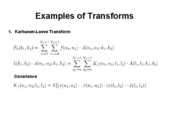
Examples of Transforms 1. Karhunen-Loeve Transform Covariance
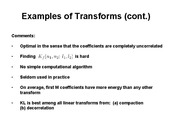
Examples of Transforms (cont. ) Comments: • Optimal in the sense that the coefficients are completely uncorrelated • Finding • No simple computational algorithm • Seldom used in practice • On average, first M coefficients have more energy than any other transform • KL is best among all linear transforms from: (a) compaction (b) decorrelation is hard
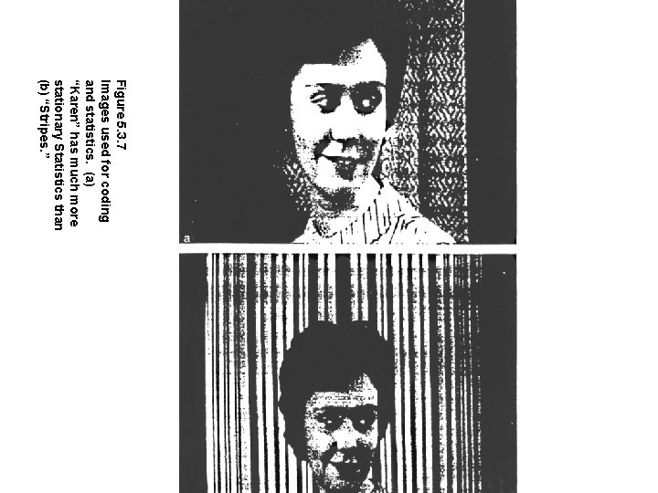
Figure 5. 3. 7 Images used for coding and statistics. (a) “Karen” has much more stationary Statistics than (b) “Stripes. ”
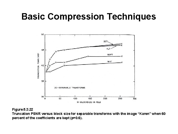
Basic Compression Techniques Figure 5. 3. 22 Truncation PSNR versus block size for separable transforms with the image “Karen” when 60 percent of the coefficients are kept (p=0. 6).
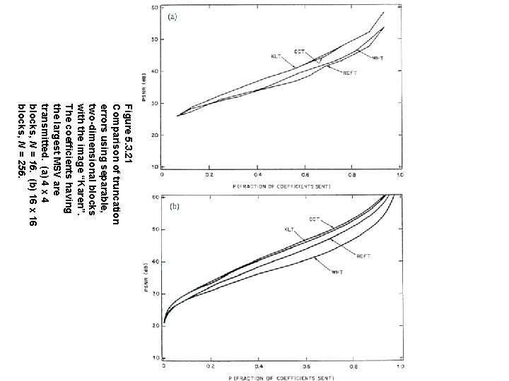
Figure 5. 3. 21 Comparison of truncation errors using separable, two-dimensional blocks with the image “Karen”. The coefficients having the largest MSV are transmitted. (a) 4 x 4 blocks, N = 16. (b) 16 x 16 blocks, N = 256.
- Slides: 61