Objective Find the line of regression Use the

Objective � Find the line of regression. � Use the Line of Regression to Make Predictions.

Relevance � To be able to find a model to best represent quantitative data with 2 variables and use it to make predictions.

2 -Variable Statistics A better alternative to “storing” numbers!

2 -Variable Statistics � Now that we have used one variable statistics to “store” our necessary numbers, let’s learn another way that’s even better

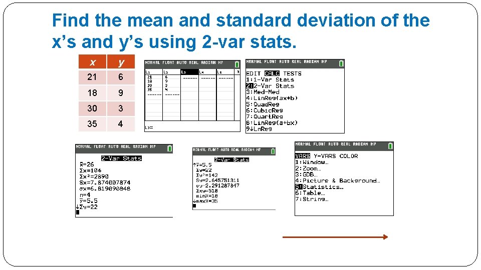
Find the mean and standard deviation of the x’s and y’s using 2 -var stats. x y 21 6 18 9 30 3 35 4

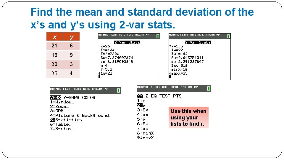
Find the mean and standard deviation of the x’s and y’s using 2 -var stats. x y 21 6 18 9 30 3 35 4 Use this when using your lists to find r.

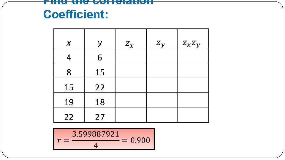
Find the correlation Coefficient: x y 4 6 8 15 22 19 18 22 27

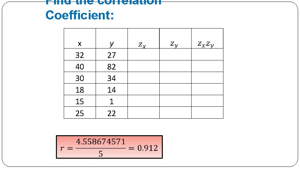
Find the correlation Coefficient: x 32 40 30 18 15 25 y 27 82 34 14 1 22

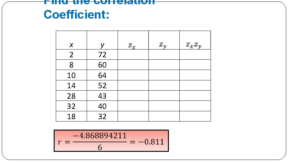
Find the correlation Coefficient: x 2 8 10 14 28 32 18 y 72 60 64 52 43 40 32

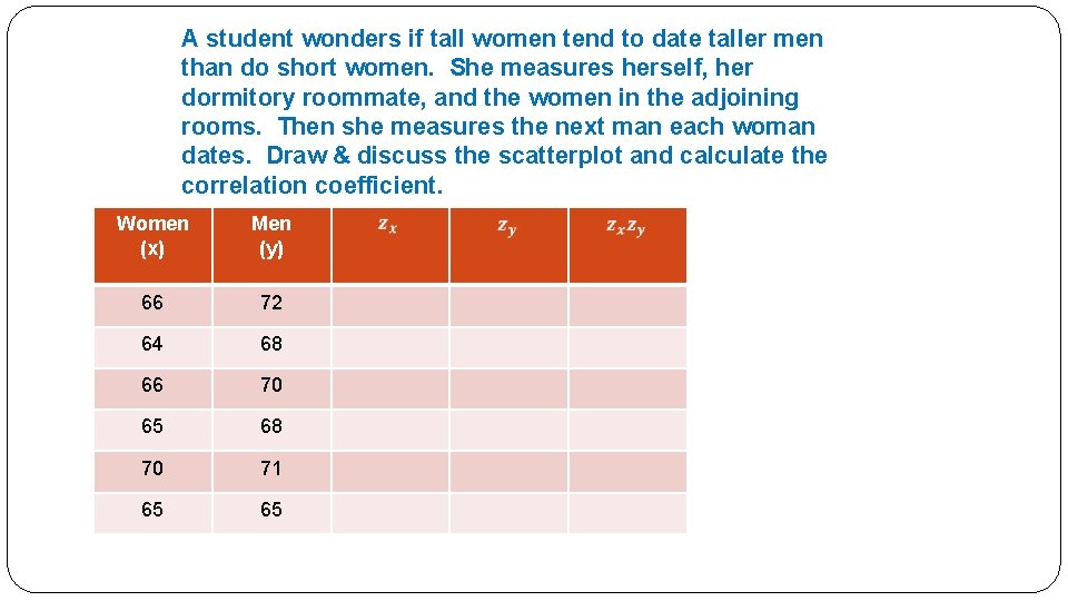
A student wonders if tall women tend to date taller men than do short women. She measures herself, her dormitory roommate, and the women in the adjoining rooms. Then she measures the next man each woman dates. Draw & discuss the scatterplot and calculate the correlation coefficient. Women (x) Men (y) 66 72 64 68 66 70 65 68 70 71 65 65

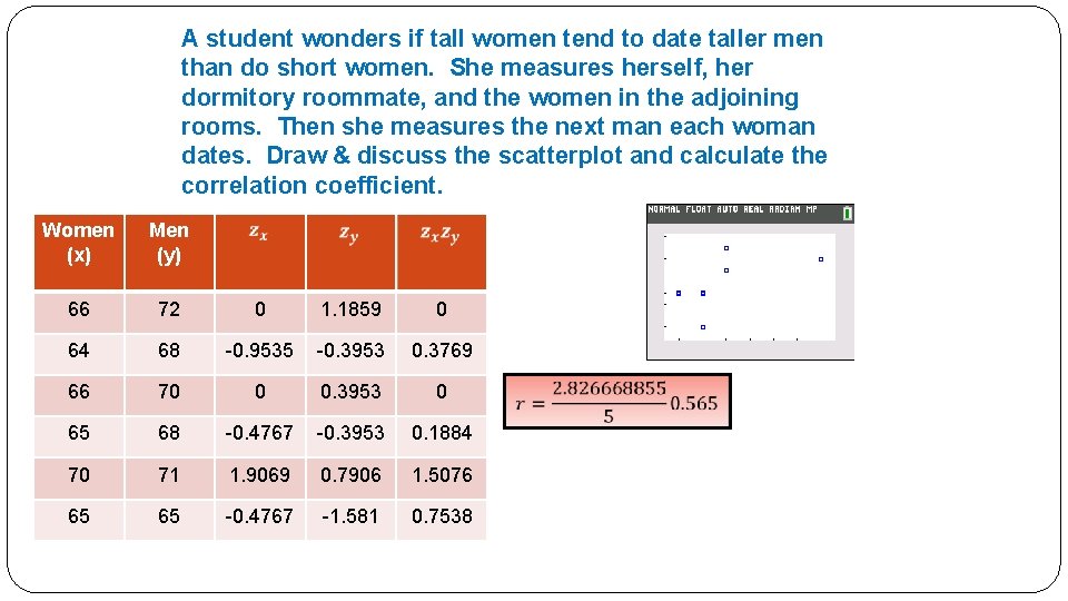
A student wonders if tall women tend to date taller men than do short women. She measures herself, her dormitory roommate, and the women in the adjoining rooms. Then she measures the next man each woman dates. Draw & discuss the scatterplot and calculate the correlation coefficient. Women (x) Men (y) 66 72 0 1. 1859 0 64 68 -0. 9535 -0. 3953 0. 3769 66 70 0 0. 3953 0 65 68 -0. 4767 -0. 3953 0. 1884 70 71 1. 9069 0. 7906 1. 5076 65 65 -0. 4767 -1. 581 0. 7538

Linear Regression

Guess the correlation coefficient �http: //istics. net/stat/Correlations/

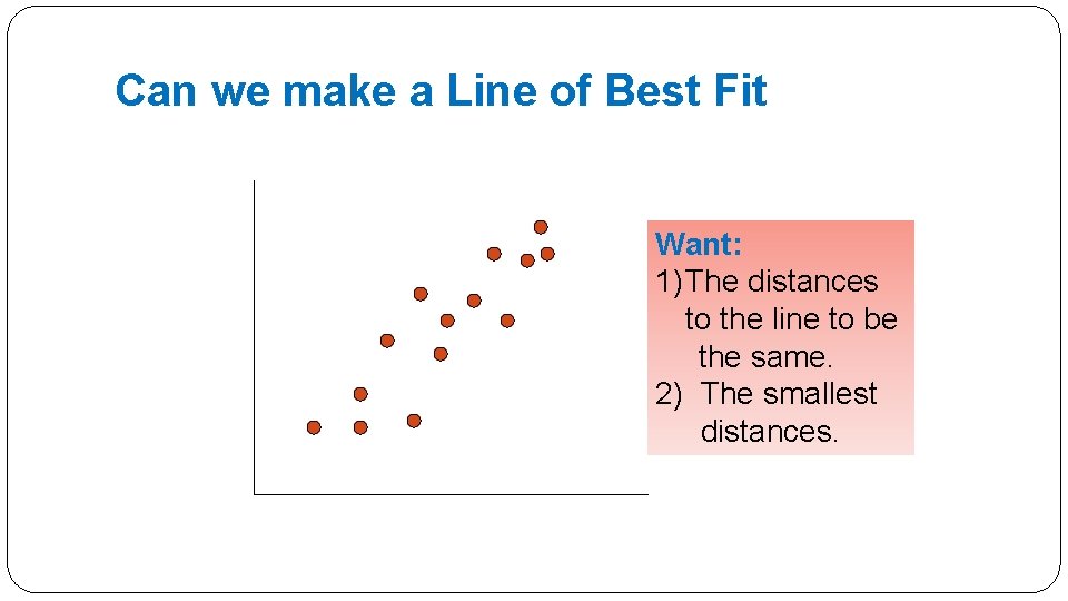
Can we make a Line of Best Fit Want: 1) The distances to the line to be the same. 2) The smallest distances.

Regression Line �When a scatterplot shows a linear relationship, we’d like to summarize the overall pattern by drawing a line on the scatterplot. �A regression line summarizes the relationship between two variables, but only in a specific setting: when one of the variables helps explain or predict the other. �Regression – unlike scatter plots – REQUIRES that we have an explanatory variable and a response variable.

Regression Line �This is a line that describes how a response variable (y) changes as an explanatory variable (x) changes. �It’s used to predict the value of (y) for a given value of (x). �The regression line is a model for the data.

Let’s try some! �http: //illuminations. nctm. org/Activity. Detail. aspx? ID=146

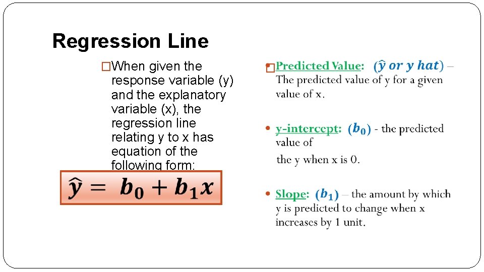
Regression Line �When given the response variable (y) and the explanatory variable (x), the regression line relating y to x has equation of the following form: �

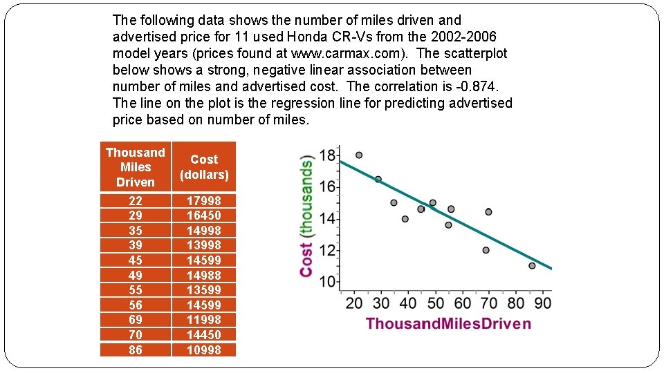
The following data shows the number of miles driven and advertised price for 11 used Honda CR-Vs from the 2002 -2006 model years (prices found at www. carmax. com). The scatterplot below shows a strong, negative linear association between number of miles and advertised cost. The correlation is -0. 874. The line on the plot is the regression line for predicting advertised price based on number of miles. Thousand Miles Driven 22 29 35 39 45 49 55 56 69 70 86 Cost (dollars) 17998 16450 14998 13998 14599 14988 13599 14599 11998 14450 10998

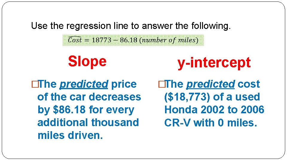
Use the regression line to answer the following. Slope �The predicted price of the car decreases by $86. 18 for every additional thousand miles driven. y-intercept �The predicted cost ($18, 773) of a used Honda 2002 to 2006 CR-V with 0 miles.

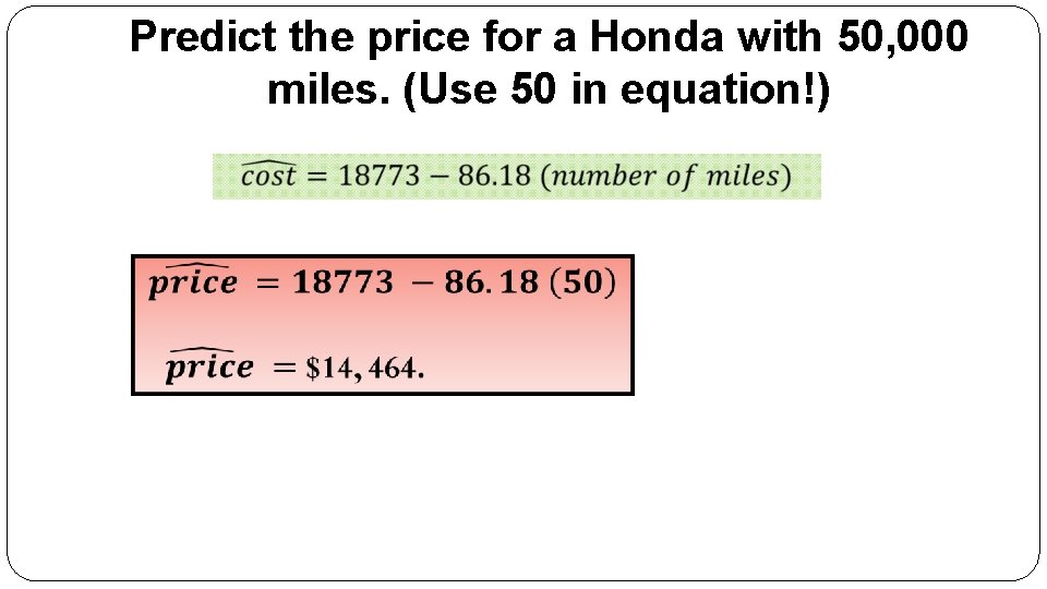
Predict the price for a Honda with 50, 000 miles. (Use 50 in equation!)

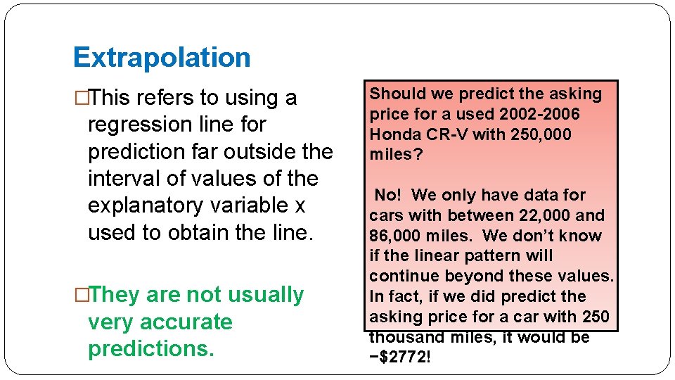
Extrapolation �This refers to using a regression line for prediction far outside the interval of values of the explanatory variable x used to obtain the line. �They are not usually very accurate predictions. Should we predict the asking price for a used 2002 -2006 Honda CR-V with 250, 000 miles? No! We only have data for cars with between 22, 000 and 86, 000 miles. We don’t know if the linear pattern will continue beyond these values. In fact, if we did predict the asking price for a car with 250 thousand miles, it would be −$2772!

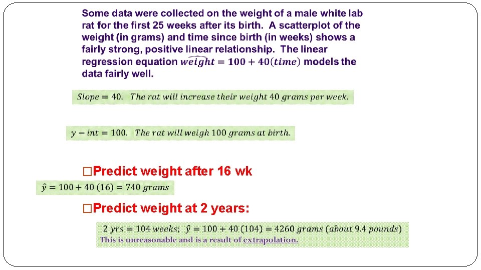
�Slope: �Y-int: �Predict weight after 16 wk �Predict weight at 2 years:

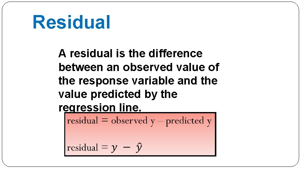
Residual A residual is the difference between an observed value of the response variable and the value predicted by the regression line.

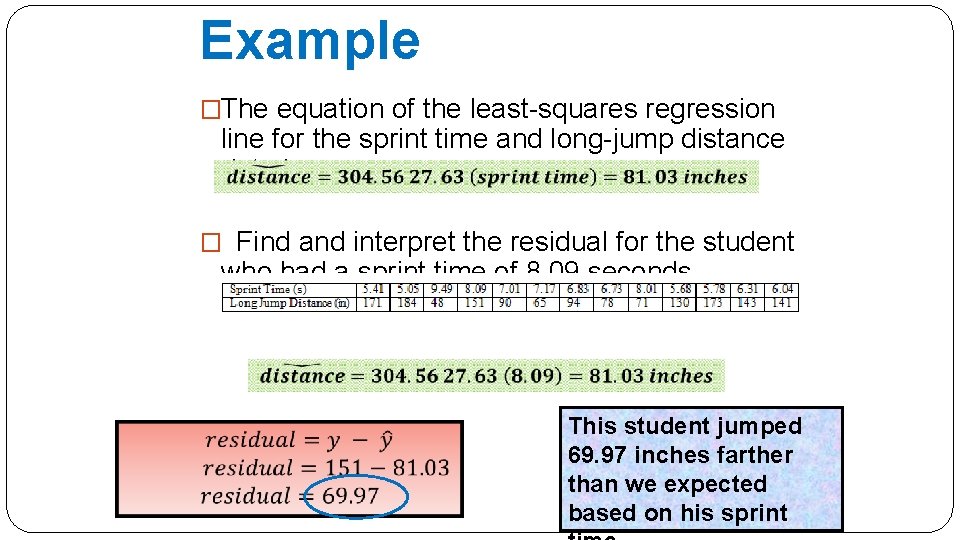
Example �The equation of the least-squares regression line for the sprint time and long-jump distance data is. � Find and interpret the residual for the student who had a sprint time of 8. 09 seconds. This student jumped 69. 97 inches farther than we expected based on his sprint

Regression �Let’s see how a regression line is calculated.

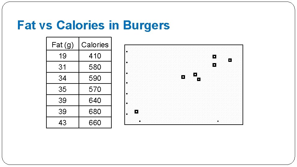
Fat vs Calories in Burgers Fat (g) 19 31 34 35 39 39 43 Calories 410 580 590 570 640 680 660

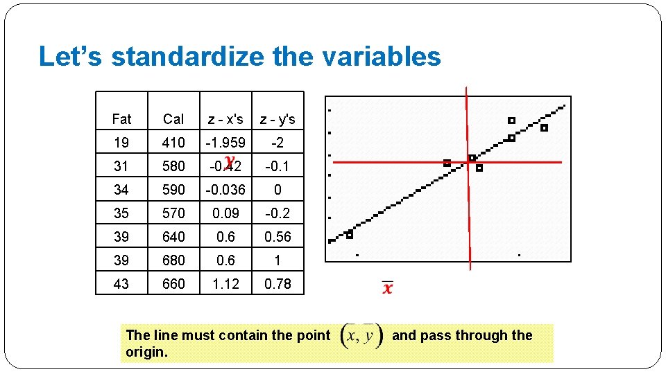
Let’s standardize the variables Fat Cal z - x's z - y's 19 410 -1. 959 -2 31 580 -0. 42 -0. 1 34 590 -0. 036 0 35 570 0. 09 -0. 2 39 640 0. 6 0. 56 39 680 0. 6 1 43 660 1. 12 0. 78 The line must contain the point origin. and pass through the

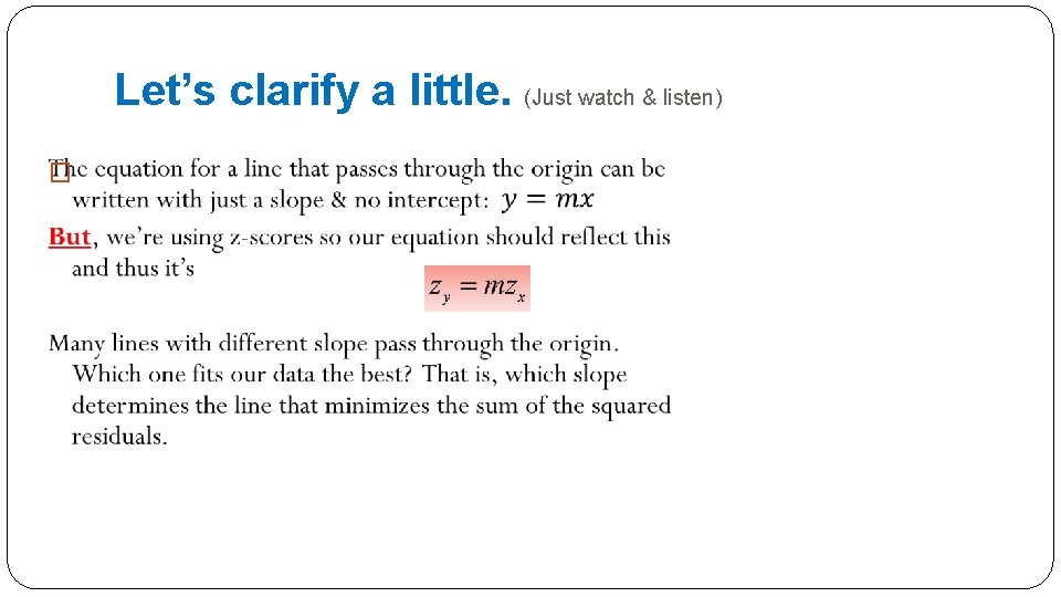
Let’s clarify a little. (Just watch & listen) �

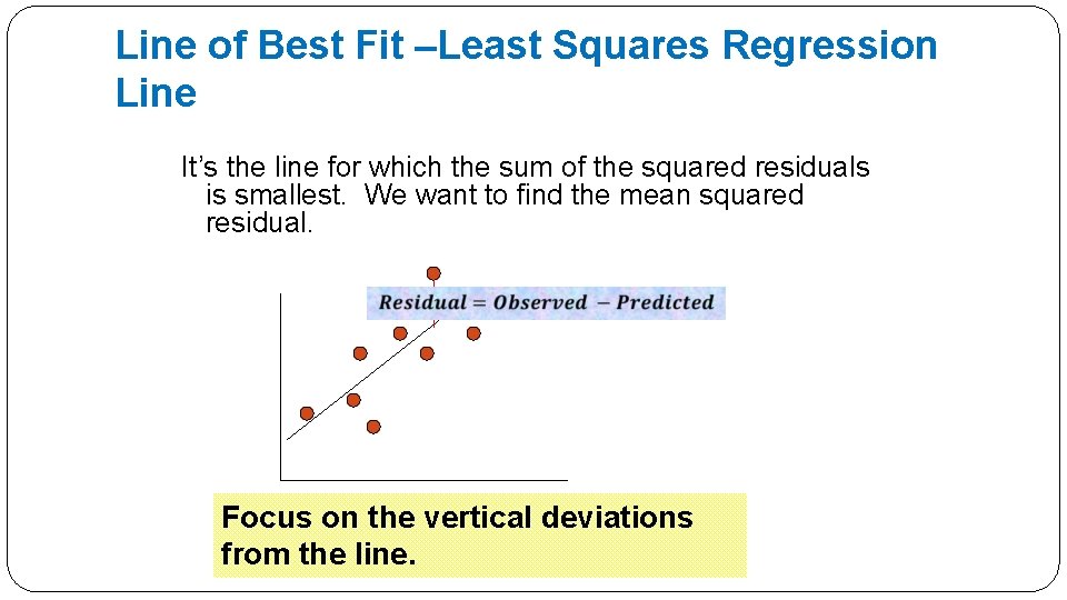
Line of Best Fit –Least Squares Regression Line It’s the line for which the sum of the squared residuals is smallest. We want to find the mean squared residual. Focus on the vertical deviations from the line.

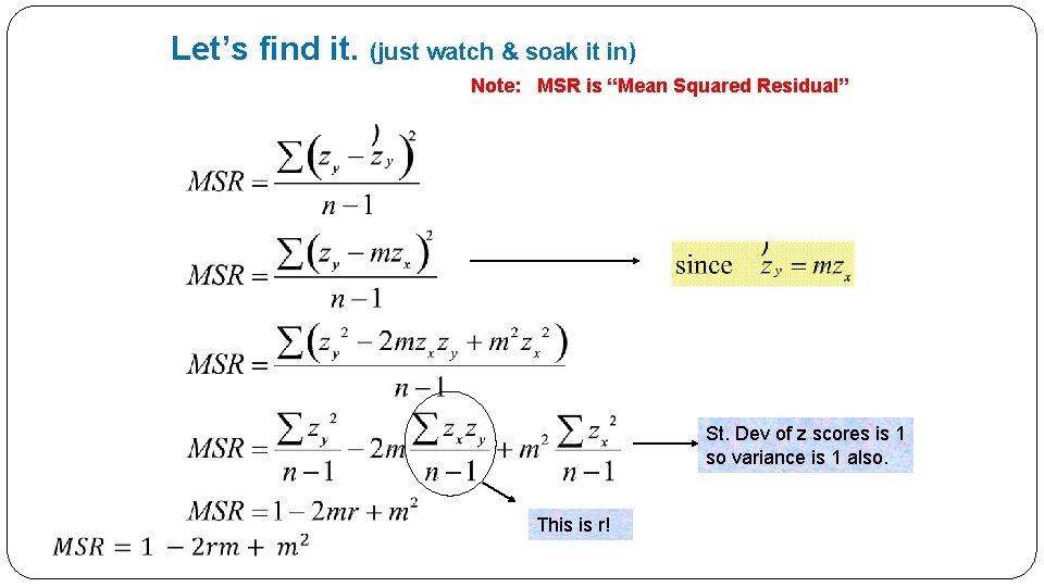
Let’s find it. (just watch & soak it in) Note: MSR is “Mean Squared Residual” St. Dev of z scores is 1 so variance is 1 also. This is r!

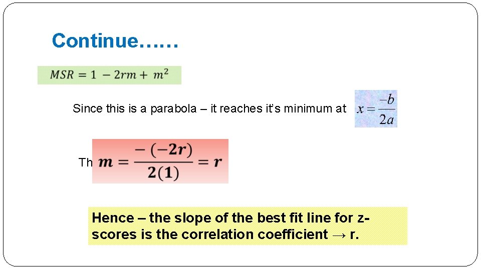
Continue…… Since this is a parabola – it reaches it’s minimum at This gives us Hence – the slope of the best fit line for zscores is the correlation coefficient → r.

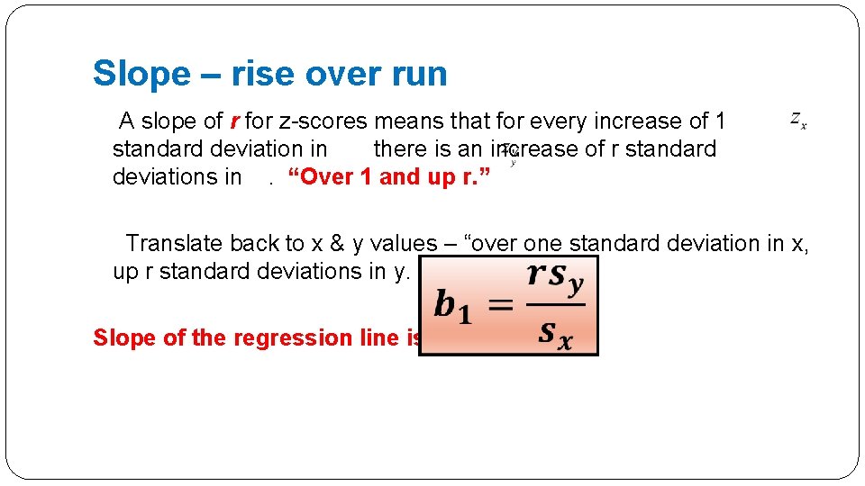
Slope – rise over run A slope of r for z-scores means that for every increase of 1 standard deviation in there is an increase of r standard deviations in . “Over 1 and up r. ” Translate back to x & y values – “over one standard deviation in x, up r standard deviations in y. Slope of the regression line is:

Why is correlation “r” �Because it was calculated from the regression of y on x after standardizing the variables – just like we have just done – thus he used r to stand for (standardized) regression.

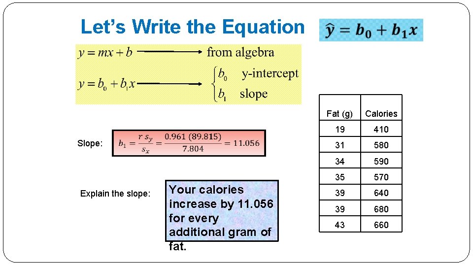
Let’s Write the Equation Slope: Explain the slope: Your calories increase by 11. 056 for every additional gram of fat. Fat (g) Calories 19 410 31 580 34 590 35 570 39 640 39 680 43 660

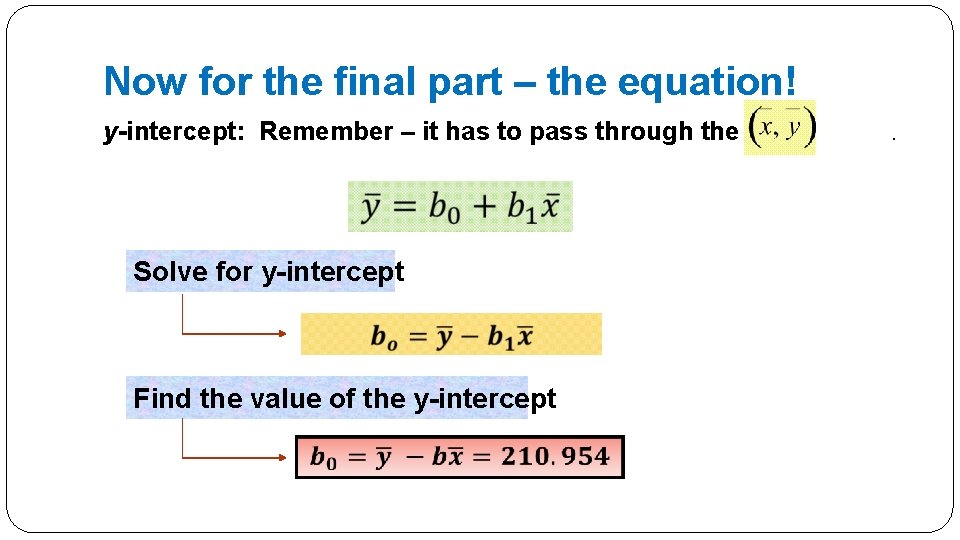
Now for the final part – the equation! y-intercept: Remember – it has to pass through the point Solve for y-intercept Find the value of the y-intercept .

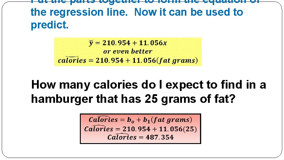
Put the parts together to form the equation of the regression line. Now it can be used to predict. How many calories do I expect to find in a hamburger that has 25 grams of fat?

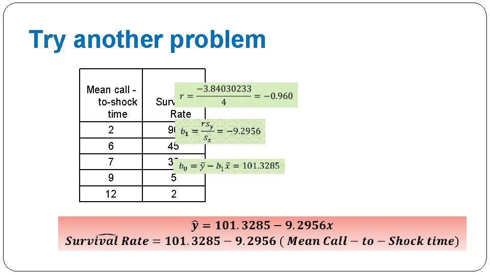
Try another problem Mean call to-shock time Survival Rate 2 90 6 45 7 30 9 5 12 2

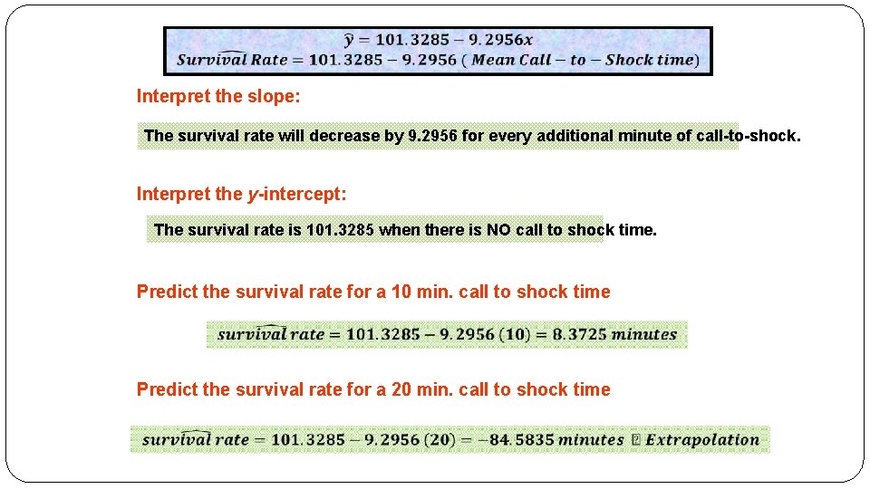
Interpret the slope: The survival rate will decrease by 9. 2956 for every additional minute of call-to-shock. Interpret the y-intercept: The survival rate is 101. 3285 when there is NO call to shock time. Predict the survival rate for a 10 min. call to shock time Predict the survival rate for a 20 min. call to shock time

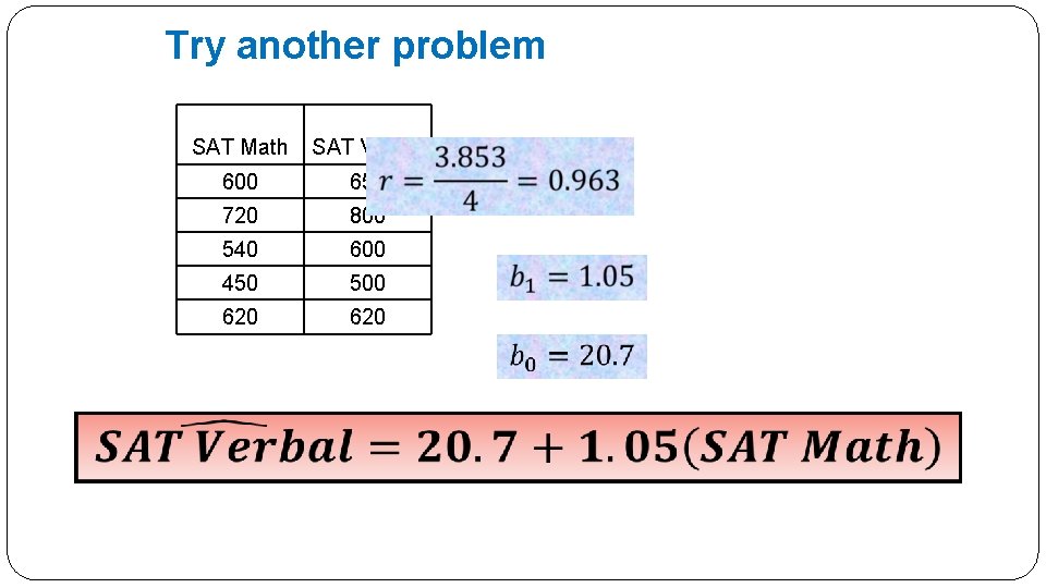
Try another problem SAT Math SAT Verbal 600 650 720 800 540 600 450 500 620

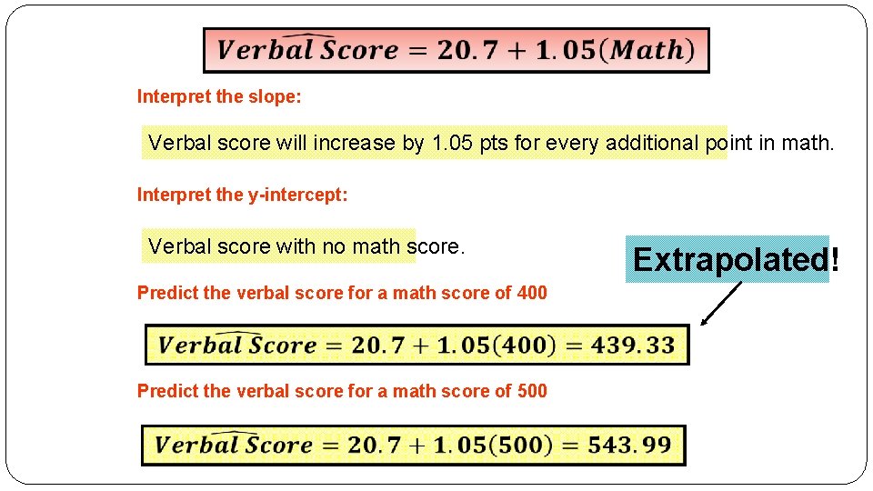
Interpret the slope: Verbal score will increase by 1. 05 pts for every additional point in math. Interpret the y-intercept: Verbal score with no math score. Predict the verbal score for a math score of 400 Predict the verbal score for a math score of 500 Extrapolated!

That’s…all…. . Folks! �Homework: p. 191 (27 -32, 35, 37, 39, 41, 47)