Object Detection Using Semi Nave Bayes to Model
Object Detection Using Semi. Naïve Bayes to Model Sparse Structure Henry Schneiderman Robotics Institute Carnegie Mellon University
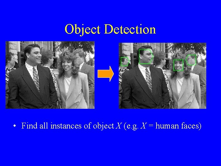
Object Detection • Find all instances of object X (e. g. X = human faces)
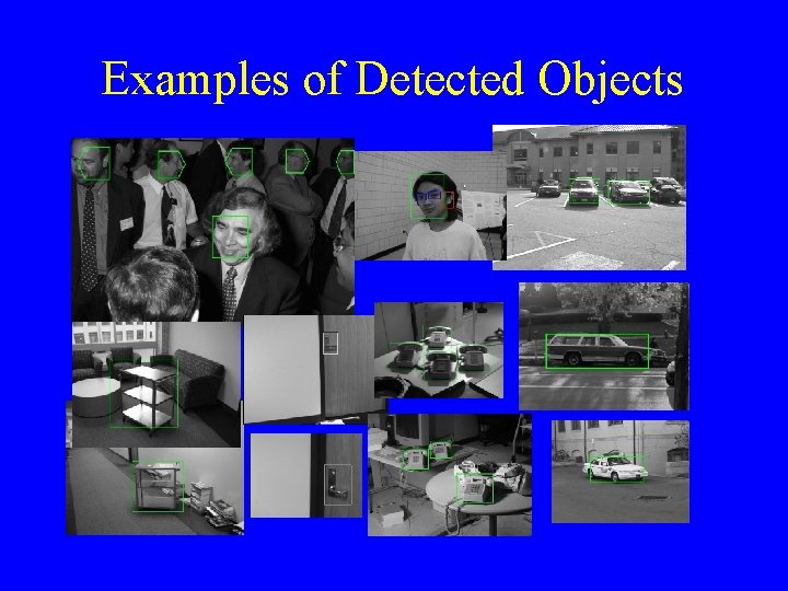
Examples of Detected Objects
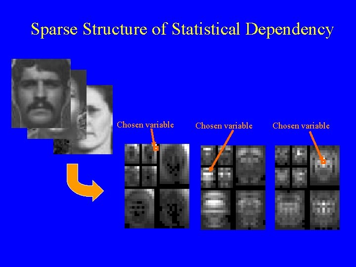
Sparse Structure of Statistical Dependency Chosen variable
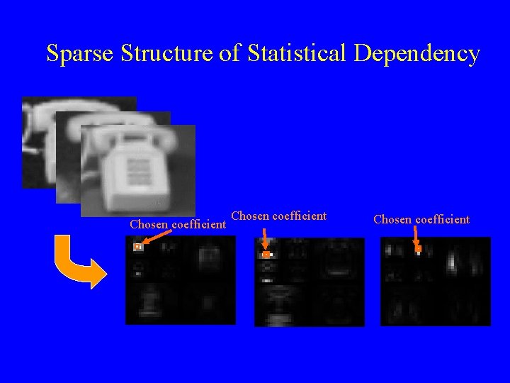
Sparse Structure of Statistical Dependency Chosen coefficient
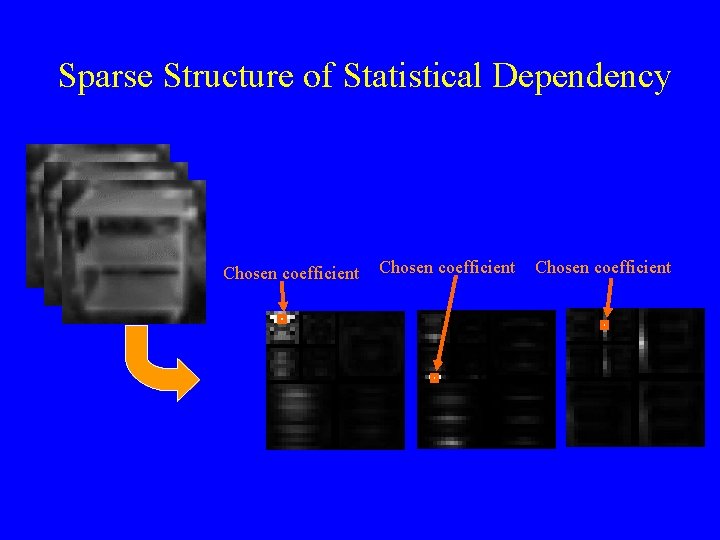
Sparse Structure of Statistical Dependency Chosen coefficient

Detection using a Classifier “Object is present” (at fixed size and alignment) Classifier “Object is NOT present” (at fixed size and alignment)
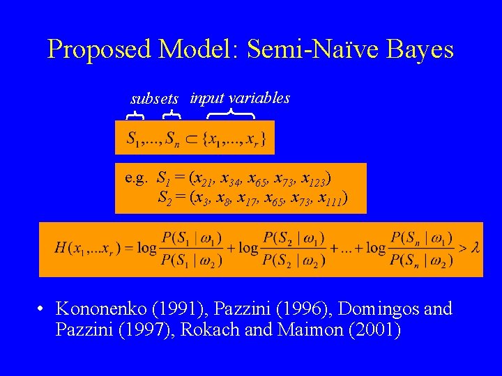
Proposed Model: Semi-Naïve Bayes subsets input variables e. g. S 1 = (x 21, x 34, x 65, x 73, x 123) S 2 = (x 3, x 8, x 17, x 65, x 73, x 111) • Kononenko (1991), Pazzini (1996), Domingos and Pazzini (1997), Rokach and Maimon (2001)
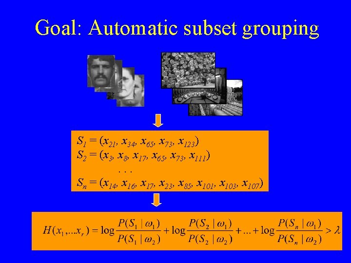
Goal: Automatic subset grouping S 1 = (x 21, x 34, x 65, x 73, x 123) S 2 = (x 3, x 8, x 17, x 65, x 73, x 111). . . Sn = (x 14, x 16, x 17, x 23, x 85, x 101, x 103, x 107)
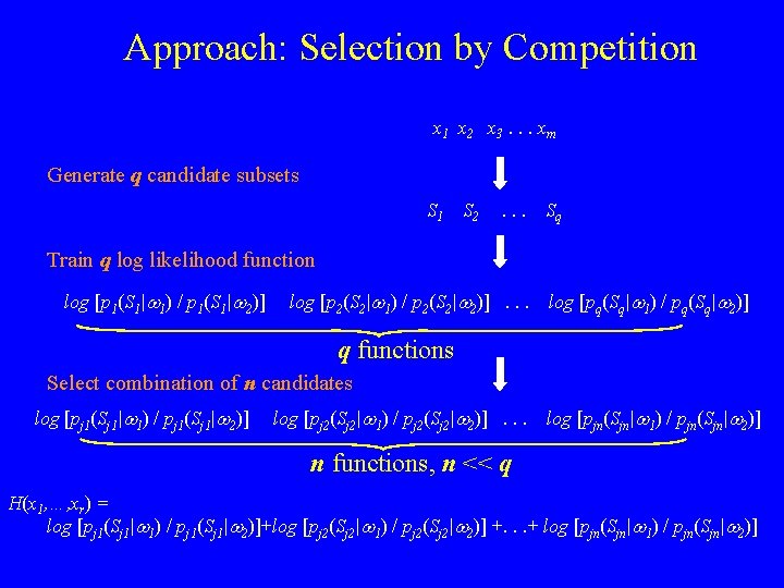
Approach: Selection by Competition x 1 x 2 x 3. . . xm Generate q candidate subsets S 1 S 2 . . . Sq Train q log likelihood function log [p 1(S 1|w 1) / p 1(S 1|w 2)] log [p 2(S 2|w 1) / p 2(S 2|w 2)]. . . log [pq(Sq|w 1) / pq(Sq|w 2)] q functions Select combination of n candidates log [pj 1(Sj 1|w 1) / pj 1(Sj 1|w 2)] log [pj 2(Sj 2|w 1) / pj 2(Sj 2|w 2)]. . . log [pjn(Sjn|w 1) / pjn(Sjn|w 2)] n functions, n << q H(x 1, …, xr) = log [pj 1(Sj 1|w 1) / pj 1(Sj 1|w 2)]+log [pj 2(Sj 2|w 1) / pj 2(Sj 2|w 2)] +. . . + log [pjn(Sjn|w 1) / pjn(Sjn|w 2)]
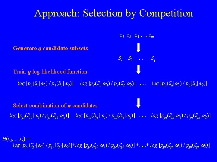
Approach: Selection by Competition x 1 x 2 x 3. . . xm Generate q candidate subsets S 1 S 2 . . . Sq Train q log likelihood function log [p 1(S 1|w 1) / p 1(S 1|w 2)] log [p 2(S 2|w 1) / p 2(S 2|w 2)]. . . log [pq(Sq|w 1) / pq(Sq|w 2)] Select combination of n candidates log [pj 1(Sj 1|w 1) / pj 1(Sj 1|w 2)] log [pj 2(Sj 2|w 1) / pj 2(Sj 2|w 2)]. . . log [pjn(Sjn|w 1) / pjn(Sjn|w 2)] H(x 1, …, xr) = log [pj 1(Sj 1|w 1) / pj 1(Sj 1|w 2)]+log [pj 2(Sj 2|w 1) / pj 2(Sj 2|w 2)] +. . . + log [pjn(Sjn|w 1) / pjn(Sjn|w 2)]
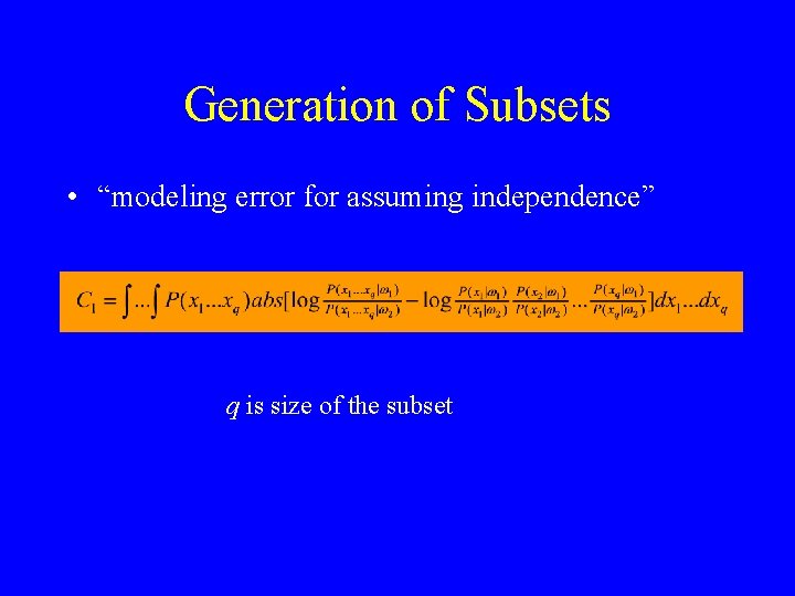
Generation of Subsets • “modeling error for assuming independence” q is size of the subset
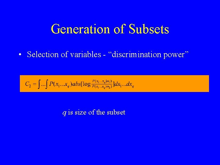
Generation of Subsets • Selection of variables - “discrimination power” q is size of the subset
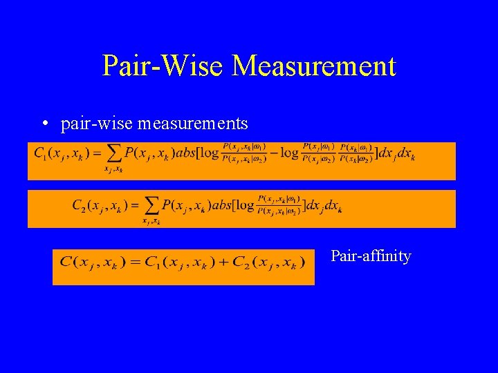
Pair-Wise Measurement • pair-wise measurements Pair-affinity
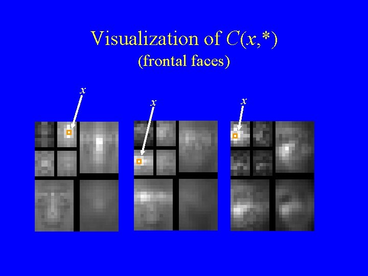
Visualization of C(x, *) (frontal faces) x x x
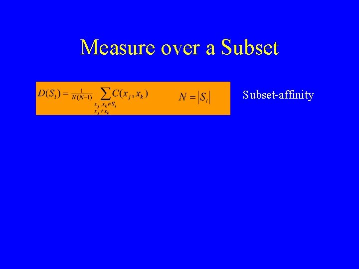
Measure over a Subset-affinity
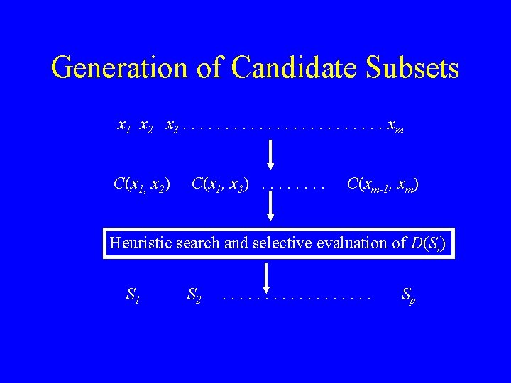
Generation of Candidate Subsets x 1 x 2 x 3. . . xm C(x 1, x 2) C(x 1, x 3). . . . C(xm-1, xm) Heuristic search and selective evaluation of D(Si) S 1 S 2 . . . . Sp
subset size vs. modeling power • Model complexity limited by number of training examples, etc. • Examples of limited modeling power – 5 modes in a mixture model – 7 projection onto principal components
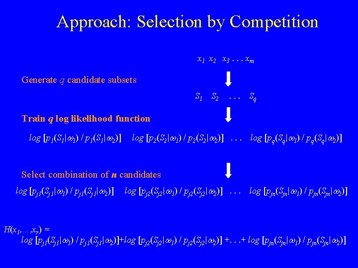
Approach: Selection by Competition x 1 x 2 x 3. . . xm Generate q candidate subsets S 1 S 2 . . . Sq Train q log likelihood function log [p 1(S 1|w 1) / p 1(S 1|w 2)] log [p 2(S 2|w 1) / p 2(S 2|w 2)]. . . log [pq(Sq|w 1) / pq(Sq|w 2)] Select combination of n candidates log [pj 1(Sj 1|w 1) / pj 1(Sj 1|w 2)] log [pj 2(Sj 2|w 1) / pj 2(Sj 2|w 2)]. . . log [pjn(Sjn|w 1) / pjn(Sjn|w 2)] H(x 1, …, xr) = log [pj 1(Sj 1|w 1) / pj 1(Sj 1|w 2)]+log [pj 2(Sj 2|w 1) / pj 2(Sj 2|w 2)] +. . . + log [pjn(Sjn|w 1) / pjn(Sjn|w 2)]
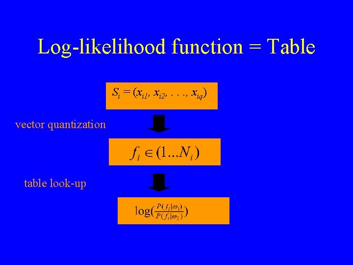
Log-likelihood function = Table Si = (xi 1, xi 2, . . . , xiq) vector quantization table look-up
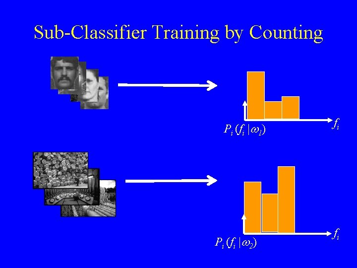
Sub-Classifier Training by Counting Pi (fi |w 1) Pi (fi |w 2) fi fi
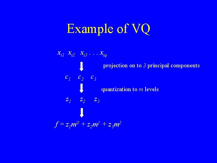
Example of VQ xi 1 xi 2 xi 3. . . xiq projection on to 3 principal components c 1 c 2 c 3 quantization to m levels z 1 z 2 z 3 f = z 1 m 0 + z 2 m 1 + z 3 m 2
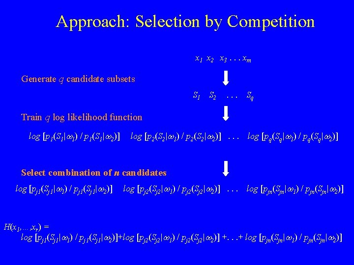
Approach: Selection by Competition x 1 x 2 x 3. . . xm Generate q candidate subsets S 1 S 2 . . . Sq Train q log likelihood function log [p 1(S 1|w 1) / p 1(S 1|w 2)] log [p 2(S 2|w 1) / p 2(S 2|w 2)]. . . log [pq(Sq|w 1) / pq(Sq|w 2)] Select combination of n candidates log [pj 1(Sj 1|w 1) / pj 1(Sj 1|w 2)] log [pj 2(Sj 2|w 1) / pj 2(Sj 2|w 2)]. . . log [pjn(Sjn|w 1) / pjn(Sjn|w 2)] H(x 1, …, xr) = log [pj 1(Sj 1|w 1) / pj 1(Sj 1|w 2)]+log [pj 2(Sj 2|w 1) / pj 2(Sj 2|w 2)] +. . . + log [pjn(Sjn|w 1) / pjn(Sjn|w 2)]
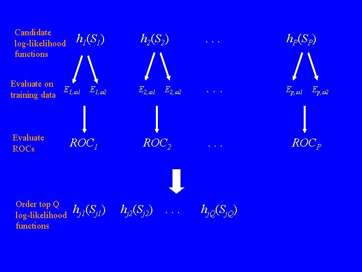
Candidate log-likelihood functions h 1(S 1) Evaluate on E training data 1, w 1 Evaluate ROCs Order top Q log-likelihood functions E 1, w 2 ROC 1 hj 1(Sj 1) h 2(S 2) . . . h. P(SP) E 2, w 1 . . . Ep, w 1 E 2, w 2 ROC 2 hj 2(Sj 2) . . . hj. Q(Sj. Q) Ep, w 2 ROCP
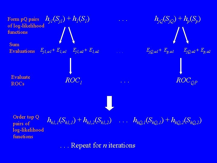
Form p. Q pairs hj 1(Sj 1) of log-likelihood functions + h 1(S 1) Sum Evaluations Ej 1, w 1+ E 1, w 1 Evaluate ROCs Order top Q pairs of log-likelihood functions Ej 1, w 2+ E 1, w 2 ROC 1 hk 1, 1(Sk 1, 1) + hk 1, 2(Sk 1, 2) . . hj. Q(Sj. Q) + hp(Sp) Ej. Q, w 1+ Ep, w 1 Ej. Q, w 2+ Ep, w 2 ROCQP . . . hk. Q, 1(Sk. Q, 1) + hk. Q, 2(Sk. Q, 2) . . . Repeat for n iterations
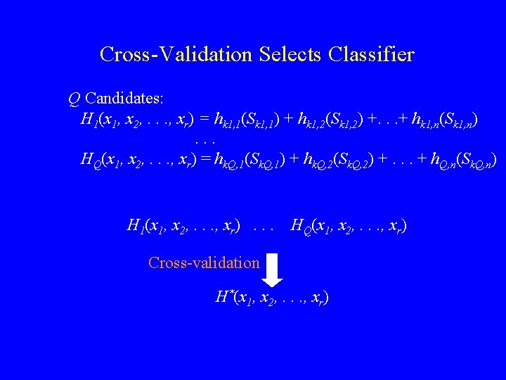
Cross-Validation Selects Classifier Q Candidates: H 1(x 1, x 2, . . . , xr) = hk 1, 1(Sk 1, 1) + hk 1, 2(Sk 1, 2) +. . . + hk 1, n(Sk 1, n). . . HQ(x 1, x 2, . . . , xr) = hk. Q, 1(Sk. Q, 1) + hk. Q, 2(Sk. Q, 2) +. . . + h. Q, n(Sk. Q, n) H 1(x 1, x 2, . . . , xr). . . HQ(x 1, x 2, . . . , xr) Cross-validation H*(x 1, x 2, . . . , xr)
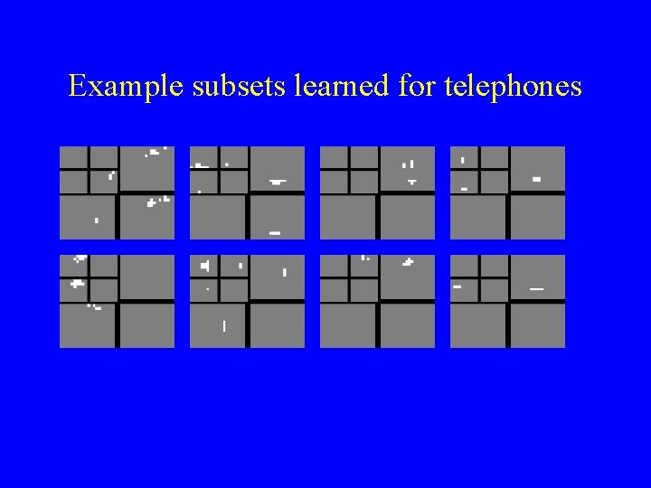
Example subsets learned for telephones
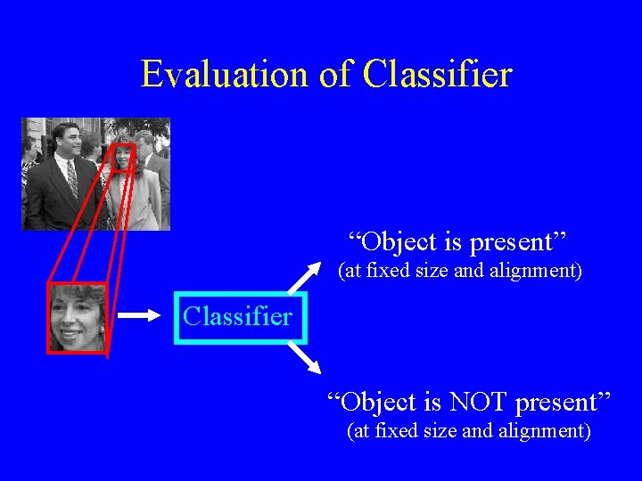
Evaluation of Classifier “Object is present” (at fixed size and alignment) Classifier “Object is NOT present” (at fixed size and alignment)
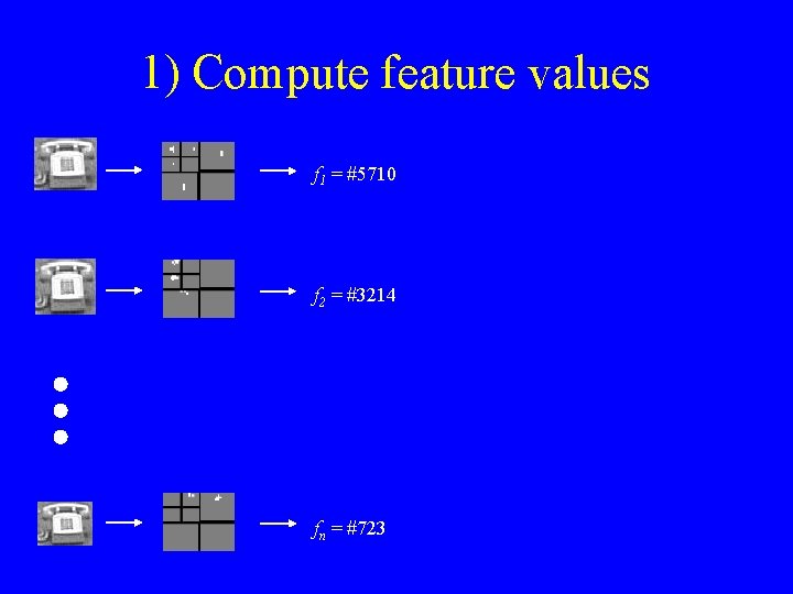
1) Compute feature values f 1 = #5710 f 2 = #3214 fn = #723
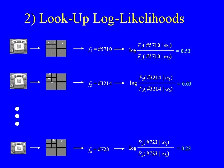
2) Look-Up Log-Likelihoods f 1 = #5710 f 2 = #3214 fn = #723 log log P 1( #5710 | w 1) P 1( #5710 | w 2) P 2( #3214 | w 1) P 2( #3214 | w 2) Pn( #723 | w 1) Pn( #723 | w 2) = 0. 53 = 0. 03 = 0. 23
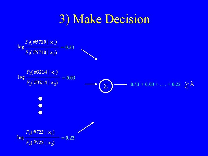
3) Make Decision log log P 1( #5710 | w 1) P 1( #5710 | w 2) P 2( #3214 | w 1) P 2( #3214 | w 2) Pn( #723 | w 1) Pn( #723 | w 2) = 0. 53 = 0. 03 S = 0. 23 0. 53 + 0. 03 +. . . + 0. 23 >l <
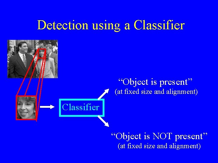
Detection using a Classifier “Object is present” (at fixed size and alignment) Classifier “Object is NOT present” (at fixed size and alignment)
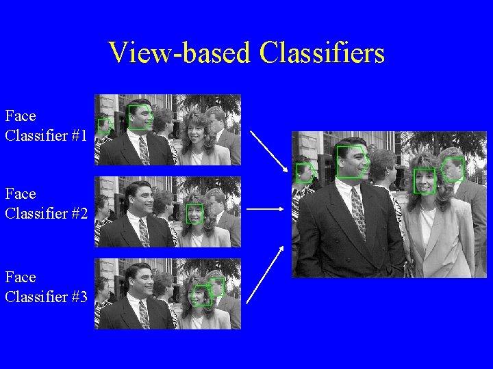
View-based Classifiers Face Classifier #1 Face Classifier #2 Face Classifier #3
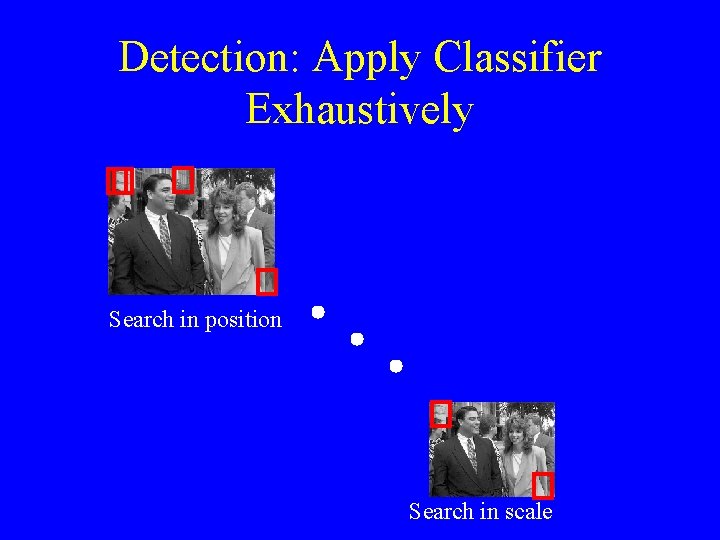
Detection: Apply Classifier Exhaustively Search in position Search in scale
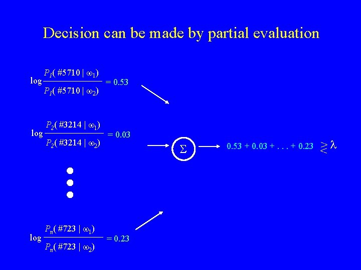
Decision can be made by partial evaluation log log P 1( #5710 | w 1) P 1( #5710 | w 2) P 2( #3214 | w 1) P 2( #3214 | w 2) Pn( #723 | w 1) Pn( #723 | w 2) = 0. 53 = 0. 03 S = 0. 23 0. 53 + 0. 03 +. . . + 0. 23 >l <
![Detection Computational Strategy Apply log [p 1(S 1|w 1) / p 1(S 1|w 2)] Detection Computational Strategy Apply log [p 1(S 1|w 1) / p 1(S 1|w 2)]](http://slidetodoc.com/presentation_image_h2/00f2890d38c447f05a32099c9f2250aa/image-36.jpg)
Detection Computational Strategy Apply log [p 1(S 1|w 1) / p 1(S 1|w 2)] exhaustively to scaled input image Apply log [p 2(S 2|w 1) / p 2(S 2|w 2)] reduced search space Computational strategy changes with size of search space Apply log [p 3(S 3|w 1) / p 3(S 3|w 2)] further reduced search space
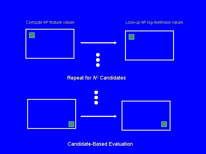
Compute M 2 feature values Look-up M 2 log-likelihood values Repeat for N 2 Candidates Candidate-Based Evaluation
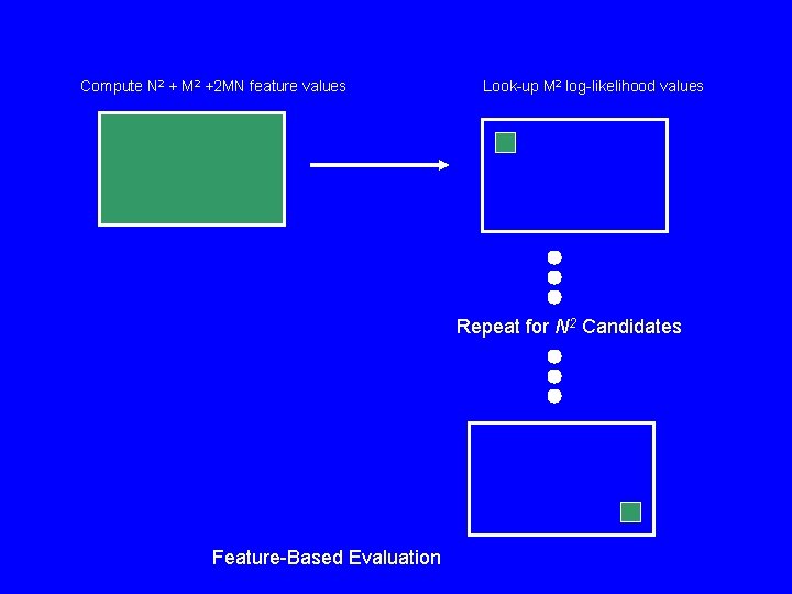
Compute N 2 + M 2 +2 MN feature values Look-up M 2 log-likelihood values Repeat for N 2 Candidates Feature-Based Evaluation
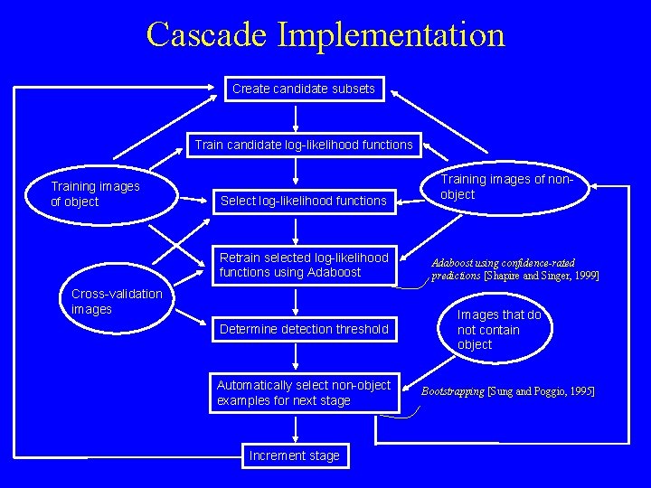
Cascade Implementation Create candidate subsets Train candidate log-likelihood functions Training images of object Select log-likelihood functions Retrain selected log-likelihood functions using Adaboost Cross-validation images Determine detection threshold Automatically select non-object examples for next stage Increment stage Training images of nonobject Adaboost using confidence-rated predictions [Shapire and Singer, 1999] Images that do not contain object Bootstrapping [Sung and Poggio, 1995]
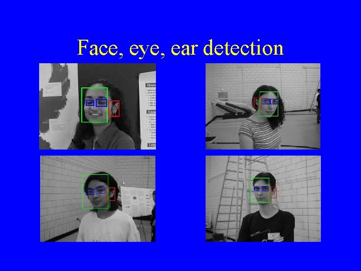
Face, eye, ear detection
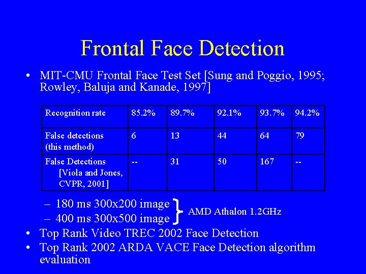
Frontal Face Detection • MIT-CMU Frontal Face Test Set [Sung and Poggio, 1995; Rowley, Baluja and Kanade, 1997] Recognition rate 85. 2% 89. 7% 92. 1% 93. 7% 94. 2% False detections (this method) 6 13 44 64 79 False Detections -[Viola and Jones, CVPR, 2001] 31 50 167 -- – 180 ms 300 x 200 image AMD Athalon 1. 2 GHz – 400 ms 300 x 500 image • Top Rank Video TREC 2002 Face Detection • Top Rank 2002 ARDA VACE Face Detection algorithm evaluation
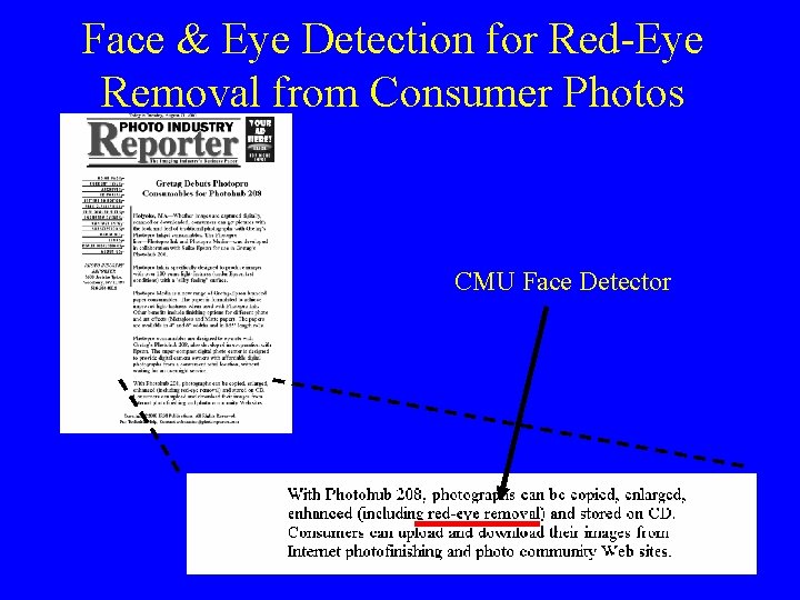
Face & Eye Detection for Red-Eye Removal from Consumer Photos CMU Face Detector
Eye Detection • Experiments performed independently at NIST • Sequested data set: 29, 627 mugshots • Eyes correctly located (radius of 15 pixels) 98. 2% (assumed one face per image) • Thanks to Jonathon Phillips, Patrick Grother, and Sam Trahan for their assistance in running these experiments
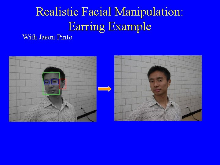
Realistic Facial Manipulation: Earring Example With Jason Pinto
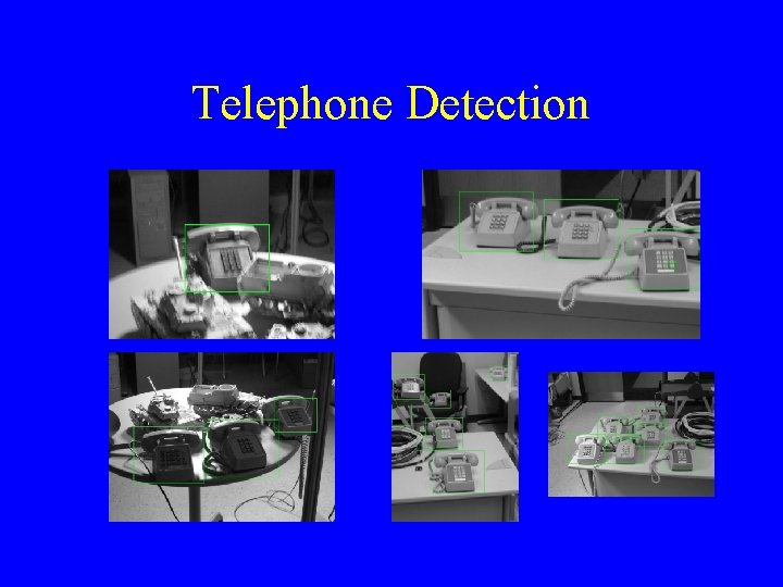
Telephone Detection
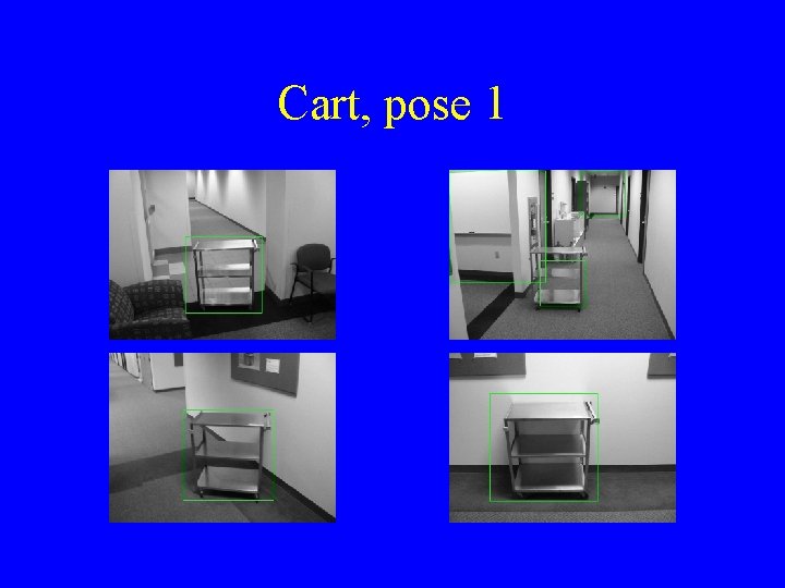
Cart, pose 1
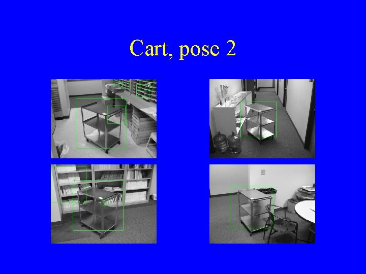
Cart, pose 2
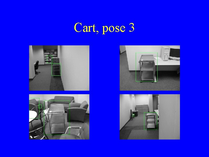
Cart, pose 3
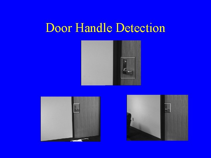
Door Handle Detection
Summary of Classifier Design • Sparse structure of statistical dependency in many image classification problem • Semi-naïve Bayes Model • Automatic learning structure of semi-naïve Bayes classifier: – Generation of many candidate subsets – Competition among many log-likelihood functions to find best combination CMU on-line face detector: http: //www. vasc. ri. cmu. edu/cgi-bin/demos/findface. cgi
- Slides: 50