NUMERICAL MODELING IN CHEMISTRY NUMERICAL KINETIC CHEMISTRY Lorentz

NUMERICAL MODELING IN CHEMISTRY • NUMERICAL KINETIC CHEMISTRY (Lorentz JÄNTSCHI, Elena Maria PICĂ) • NUMERICAL DESCRIPTION OF TITRATION (Lorentz JÄNTSCHI, Horea Iustin NAŞCU) • CORRELATIONS AND REGRESSIONS WITH MATHLAB (Lorentz JÄNTSCHI, Mihaela UNGUREŞAN)

NUMERICAL KINETIC CHEMISTRY (Lorentz JÄNTSCHI, Elena Maria PICĂ)

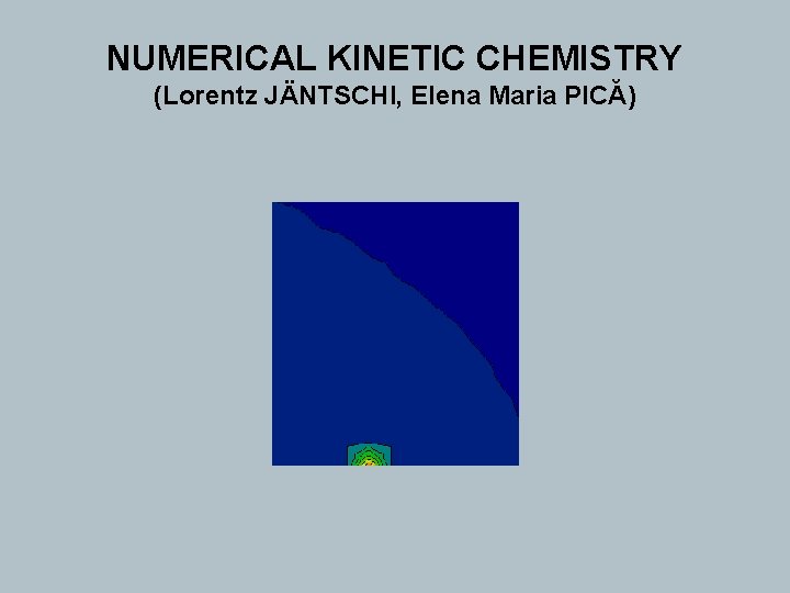
Concentration gradient in an oscillating reaction The oscillating reactions are more than a laboratory curiosity. If in the industrial processes they appear in few cases, in biochemical systems there are numerous examples of oscillating reactions. For instance, the oscillating reactions maintain the rhythm. All live processes are based on one or more oscillating reactions.

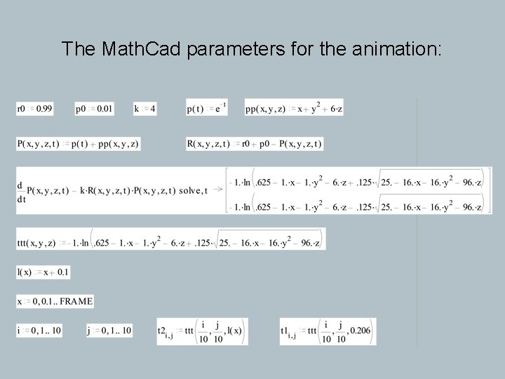
The Math. Cad parameters for the animation:

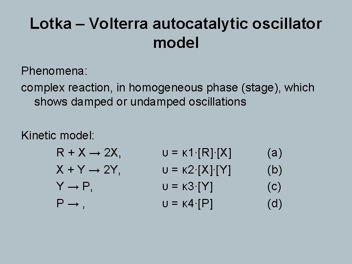
Lotka – Volterra autocatalytic oscillator model Phenomena: complex reaction, in homogeneous phase (stage), which shows damped or undamped oscillations Kinetic model: R + X → 2 X, X + Y → 2 Y, Y → P, P→, υ = κ 1·[R]·[X] υ = κ 2·[X]·[Y] υ = κ 3·[Y] υ = κ 4·[P] (a) (b) (c) (d)

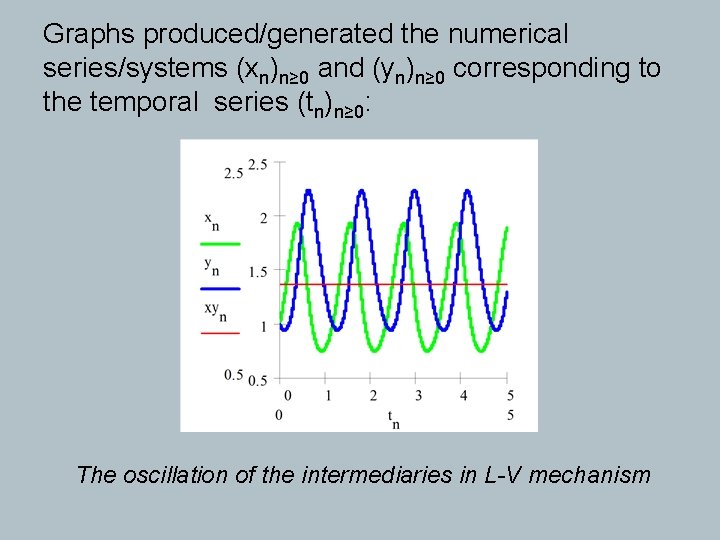
Mathematical model: = υ(a) − υ(b) = κ 1·[R]·[X] − κ 2·[X]·[Y] (1) = υ(b) − υ(c) = κ 2·[X]·[Y] − κ 3·[Y] (2) Numerical model: xn+1 = xn+ (tn+1 -tn)·xn·(κ 1·[R]-κ 2·yn) (3) yn+1 = yn+(tn+1 -tn)·yn·(κ 2·xn-κ 3) (4) x 0 = [X]0 = 1, y 0 = [Y]0 = 1, κ 1 = 3, κ 2 = 4, κ 3 = 5, [R] = 2

Graphs produced/generated the numerical series/systems (xn)n≥ 0 and (yn)n≥ 0 corresponding to the temporal series (tn)n≥ 0: The oscillation of the intermediaries in L-V mechanism

The variation path ([X], [Y]) in the L-V mechanism

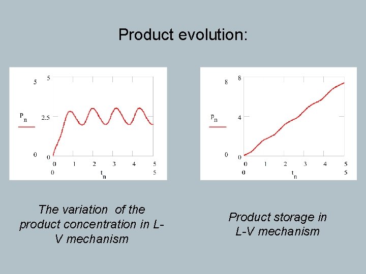
Product evolution: The variation of the product concentration in LV mechanism Product storage in L-V mechanism

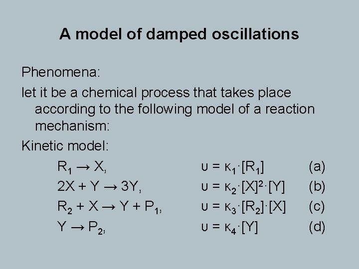
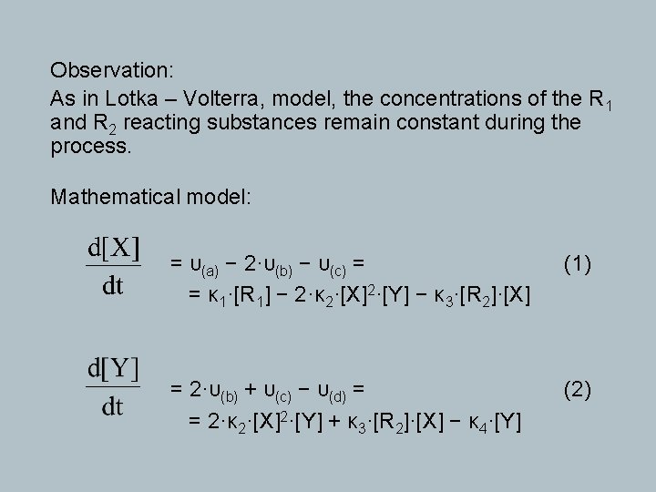
A model of damped oscillations Phenomena: let it be a chemical process that takes place according to the following model of a reaction mechanism: Kinetic model: R 1 → X, υ = κ 1·[R 1] (a) 2 X + Y → 3 Y, υ = κ 2·[X]2·[Y] (b) R 2 + X → Y + P 1, υ = κ 3·[R 2]·[X] (c) Y → P 2, υ = κ 4·[Y] (d)

Observation: As in Lotka – Volterra, model, the concentrations of the R 1 and R 2 reacting substances remain constant during the process. Mathematical model: = υ(a) − 2·υ(b) − υ(c) = = κ 1·[R 1] − 2·κ 2·[X]2·[Y] − κ 3·[R 2]·[X] (1) = 2·υ(b) + υ(c) − υ(d) = = 2·κ 2·[X]2·[Y] + κ 3·[R 2]·[X] − κ 4·[Y] (2)

Numerical model: xn+1 = xn+(tn+1 -tn)·(κ 1·[R 1]-xn·(2·κ 2·xn·yn+κ 3·[R 2])) (3) yn+1 = yn+(tn+1 -tn)·(xn·(2·κ 2·xn·yn+κ 3·[R 2])-κ 4·yn) (4) Data output: x 0 = 0, y 0 = 1, κ 1 = 3, κ 2 = 4, κ 3 = 5, κ 4 = 7, [R 1] = 2, [R 2] = 2, tn = n/100000 with n = 0, 1. . 300000

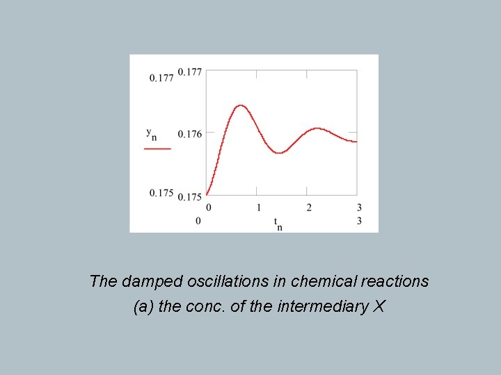
The damped oscillations in chemical reactions (a) the conc. of the intermediary X

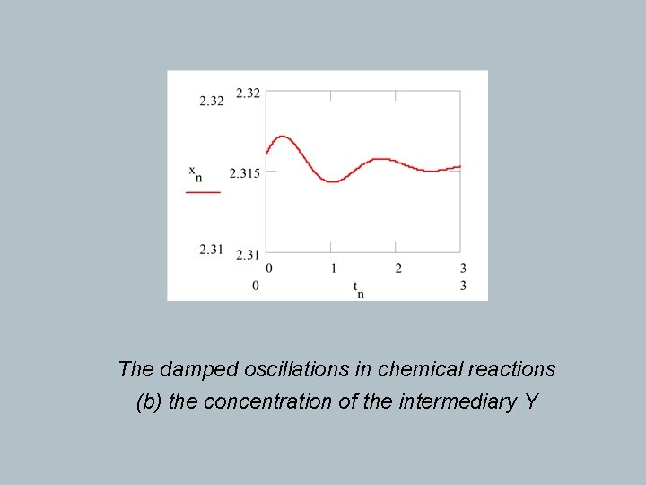
The damped oscillations in chemical reactions (b) the concentration of the intermediary Y

The damped oscillations in chemical reactions (c) the damped oscillation path ([X], [Y])

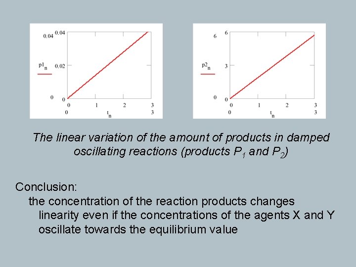
Data results: equilibrium concentration are [X] = 2. 315 and [Y] = 0. 176 and the equilibrium ratio are [X]/[Y] = 13. 53 the dependence on time (tn)n≥ 0 of the accumulation of the reaction products [P 1] = (p 1 n)n≥ 0 and [P 2] = (p 2 n)n≥ 0 is linear (see next graphs)

The linear variation of the amount of products in damped oscillating reactions (products P 1 and P 2) Conclusion: the concentration of the reaction products changes linearity even if the concentrations of the agents X and Y oscillate towards the equilibrium value

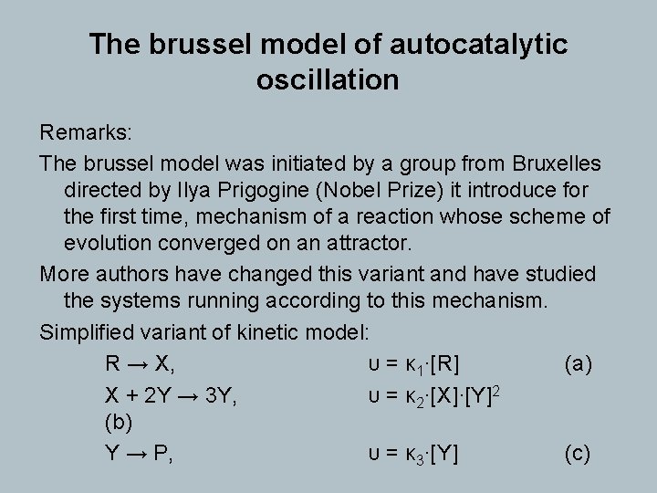
The brussel model of autocatalytic oscillation Remarks: The brussel model was initiated by a group from Bruxelles directed by Ilya Prigogine (Nobel Prize) it introduce for the first time, mechanism of a reaction whose scheme of evolution converged on an attractor. More authors have changed this variant and have studied the systems running according to this mechanism. Simplified variant of kinetic model: R → X, υ = κ 1·[R] (a) X + 2 Y → 3 Y, υ = κ 2·[X]·[Y]2 (b) Y → P, υ = κ 3·[Y] (c)

Mathematical model: = υ(a) − υ(b) = κ 1·[R 1] − κ 2·[X]·[Y]2 (1) = υ(b) − υ(c) = κ 2·[X]·[Y]2 − κ 3·[Y] (2) Observations: Though the equations (1) and (2) seem simpler, at first sight, they are even more difficult to be solved by integration than previous cases. Moreover, the literature has not recorded their integration into the general case described by (1 -2). Besides, the equations do not lead to an attractor model not matter by values of the constants of speed and of the concentrations [R], [X]0 and [Y]0.

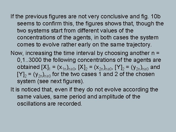
The attempt of solving (1 -2) is full of surprises. For most of the values a system which develops towards a position of equilibrium is obtained; there are values for which damped oscillations to equilibrium are found again; the undamped periodical oscillations have also an important role, which is confirmed by the majority of the organisms in which the cellular biochemical processes are based on such oscillations. The processes taking place within the heart are a conclusive example; the periodical heart beats are due to processes of this type. The importance of these processes is great. This was the reason for which Ilya Prigogine was awarded the Nobel Prize for chemistry in 1977, namely for his theories on the dissipative systems.

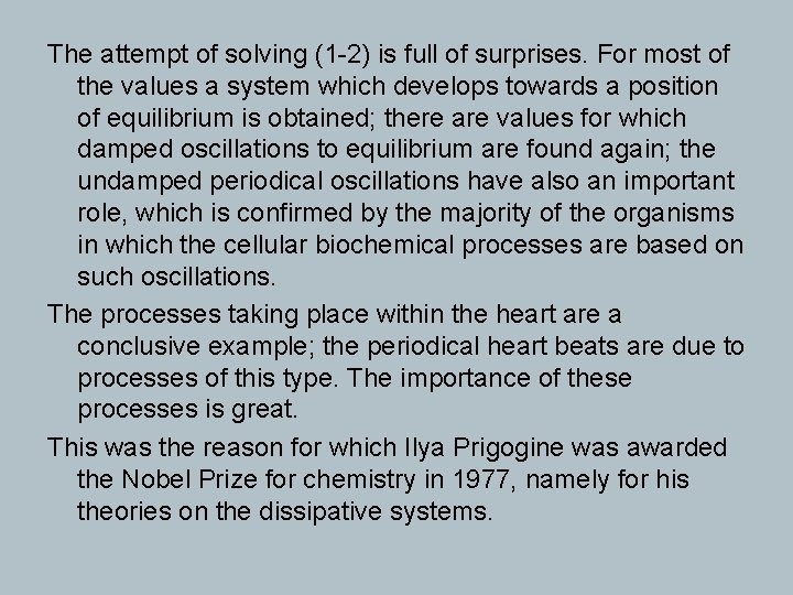
The equations (1 -2) are simplified if [R] = 1, κ 1 = 1 and κ 3 = 1, are chosen and when the differential system of equations becomes: x’ = 1 – κ 2·x·y 2; y’ = κ 2·x·y 2 – y (3) However, the numerical simulation is made in the same way. Thus the iteration equation of variation for (3) is written: xn+1 = xn+(tn+1 -tn)·(1 -κ 2·xn·yn 2), yn+1 = yn+(tn+1 -tn)·(κ 2·xn·yn 2 -yn) (4) Now choosing κ 2 = 0. 88 and taking into consideration two cases, the first one in which the initial concentrations of the agents are x 10 = [X]1, 0 = 1. 5 and y 10 = [Y]1, 0 = 2 and second case in which x 20 = [X]2, 0 = 2 and y 20 = [Y]2, 0 = 2. 5 and the series tn = n/100 with n = 0, 1. . 150,

following representations for the concentrations of the agents [X] = (xn)n≥ 0 and [Y] = (yn)n≥ 0 are obtained: The concentrations of the intermediaries up to the attractor for two cases with different I. C.

And the variation diagram of [Y] depending on [X] and the variation in time of the storage of reaction product is: (a) The entrance of [Y] related to [X] on the same gravitational orbit for (b) different product quantities obtained in two cases having different initial conditions

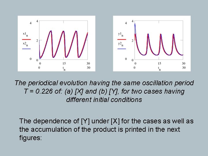
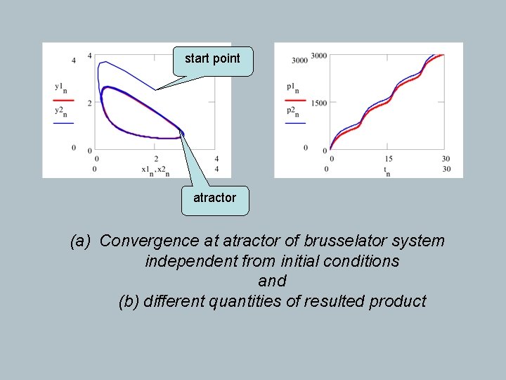
If the previous figures are not very conclusive and fig. 10 b seems to confirm this, the figures shows that, though the two systems start from different values of the concentrations of the agents, in both cases the system comes to evolve rather early on the same trajectory. Now, increasing the time interval by choosing another n = 0, 1. . 3000 the following concentrations of the agents are obtained [X]1 = (x 1 n)n≥ 0, [X]2 = (x 2 n)n≥ 0, [Y]2 = (y 2 n)n≥ 0 and [Y]2 = (y 2 n)n≥ 0 for the two cases 1 and 2 of the chosen system (see next figures). It is noticed that, even if they do not evolve according the same values, same period and amplitude of the oscillations are recorded.

The periodical evolution having the same oscillation period T = 0. 226 of: (a) [X] and (b) [Y], for two cases having different initial conditions The dependence of [Y] under [X] for the cases as well as the accumulation of the product is printed in the next figures:

start point atractor (a) Convergence at atractor of brusselator system independent from initial conditions and (b) different quantities of resulted product

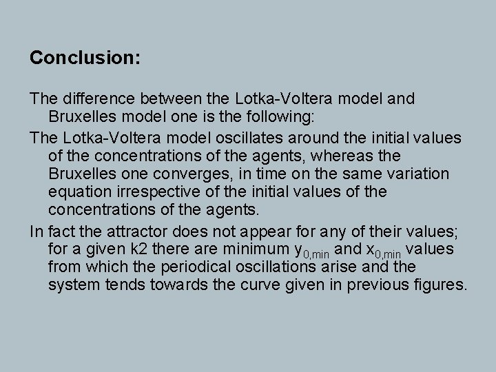
Conclusion: The difference between the Lotka-Voltera model and Bruxelles model one is the following: The Lotka-Voltera model oscillates around the initial values of the concentrations of the agents, whereas the Bruxelles one converges, in time on the same variation equation irrespective of the initial values of the concentrations of the agents. In fact the attractor does not appear for any of their values; for a given k 2 there are minimum y 0, min and x 0, min values from which the periodical oscillations arise and the system tends towards the curve given in previous figures.

References: M. Diudea, I. Gutman, L. Jäntschi (2001), Molecular Topology, Nova Science, Huntington, New York, 332 p. , ISBN 1 -56072 -957 -0. M. V. Diudea, Ed. (2001), QSPR / QSAR Studies by Molecular Descriptors, Nova Science, Huntington, New York, 438 p. , ISBN 1 -56072 -859 -0. L. Jäntschi, M. Ungureşan (2001), Chimie Fizică. Cinetică şi Dinamică Moleculară, Mediamira, Cluj-Napoca, 159 p. , ISBN 973 -9358 -71 -3. L. Jäntschi (2002), Studii Fitosanitare, Amici, Cluj-Napoca, 140 p. , in press.

NUMERICAL DESCRIPTION OF TITRATION (Lorentz JÄNTSCHI, Horea Iustin NAŞCU) Abstract: The analytical methods of qualitative and quantitative determination of ions in solutions are very flexible to automation. The process of titration is a recurrent process that can be watched by permanent measurement of a simple property such as mass, current intensity, tension, volume or a complex property such as adsorption, heat of reaction, which need a complex evaluation. The present work is focused on modeling the process of titration and presents a numerical simulation of acid-base titration. Titration parameter selected is the p. H. The method permits to observe the titration process and identify the equivalence point of titration.

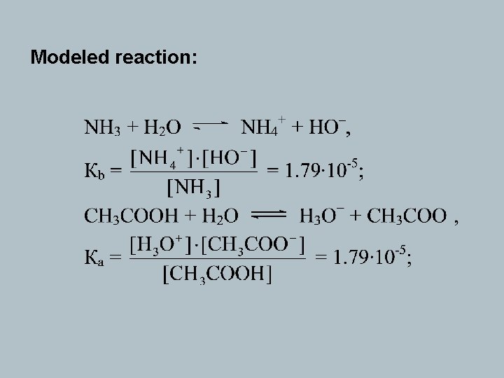
Modeled reaction:

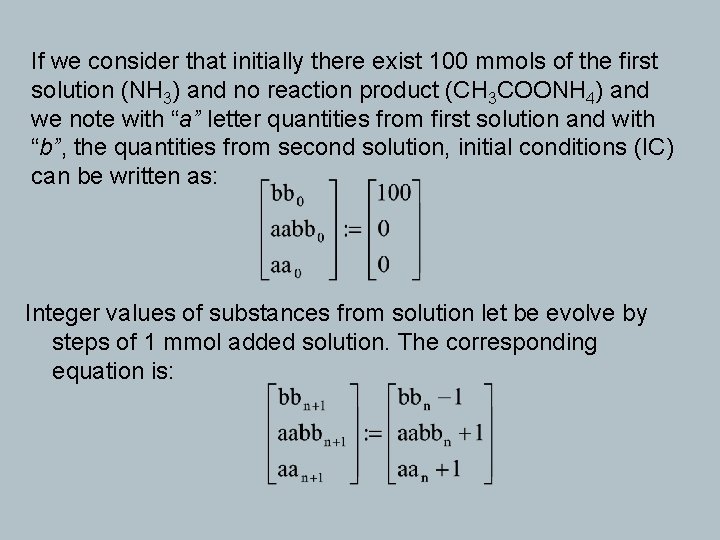
If we consider that initially there exist 100 mmols of the first solution (NH 3) and no reaction product (CH 3 COONH 4) and we note with “a” letter quantities from first solution and with “b”, the quantities from second solution, initial conditions (IC) can be written as: Integer values of substances from solution let be evolve by steps of 1 mmol added solution. The corresponding equation is:

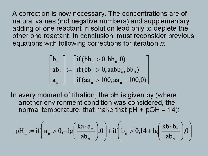
A correction is now necessary. The concentrations are of natural values (not negative numbers) and supplementary adding of one reactant in solution lead only to deplete the other one reactant. In conclusion, must reconsider previous equations with following corrections for iteration n: In every moment of titration, the p. H is given by (where another environment condition was considered, the normal temperature, that make that p. H + p. OH = 14):

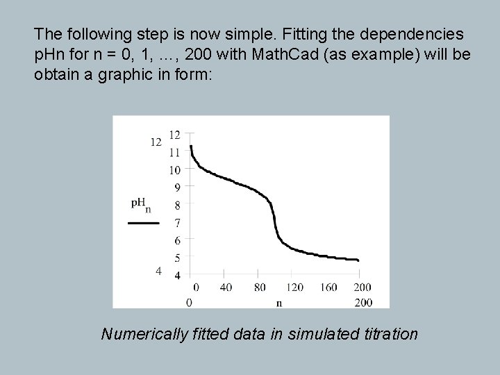
The following step is now simple. Fitting the dependencies p. Hn for n = 0, 1, …, 200 with Math. Cad (as example) will be obtain a graphic in form: Numerically fitted data in simulated titration

Conclusions and remarks The titration process is simple in appearance but shows to be complex in details. Even the simple case of titration of monobasic base ammonia with a monoprotic acid, such as acetic acid, hangs up unexpected difficulties in simulation process. The difficulties exists especially because is no approximations in model. Only one (so called) approximation is sequent adding of titrate, that are also perfectly possible in practice. The method permits to investigate more complex processes such as titration of polyprotic acids and polybasic bases. If no approximation will be made, more complex equations will be necessary and superior rank equations will appear to be solved.

CORRELATIONS AND REGRESSIONS WITH MATHLAB (Lorentz JÄNTSCHI, Mihaela UNGUREŞAN) Abstract: A MATHLab computer program is implemented. The program presented demonstrates the power of MATHLab in working with statistical processing, and can be considered as an example for future applications. The program draws an exportable figure of fitted data and regression curve and calculates the correlation coefficient r and sum of residues.

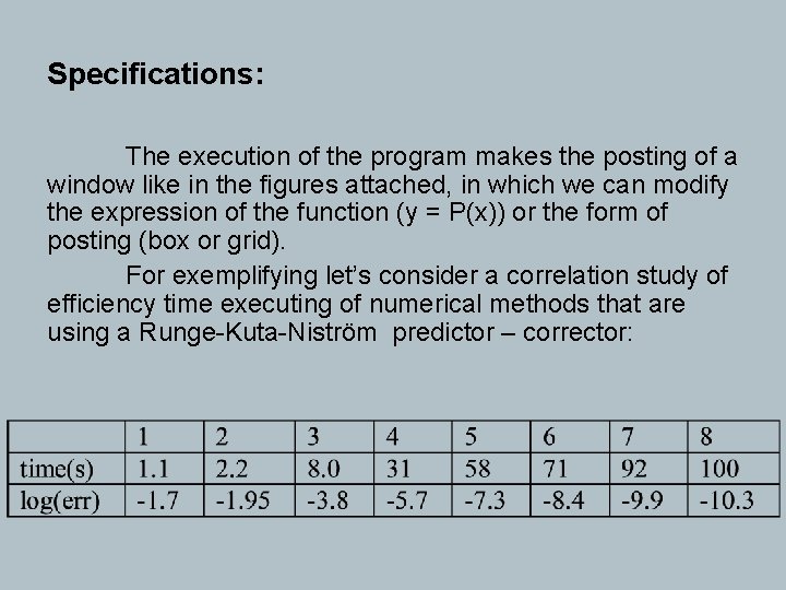
Specifications: The execution of the program makes the posting of a window like in the figures attached, in which we can modify the expression of the function (y = P(x)) or the form of posting (box or grid). For exemplifying let’s consider a correlation study of efficiency time executing of numerical methods that are using a Runge-Kuta-Niström predictor – corrector:

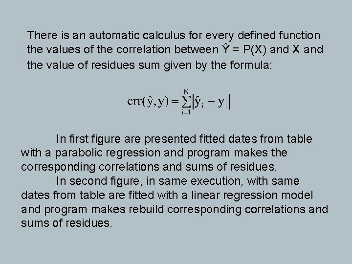
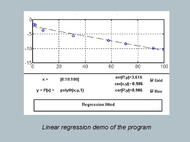
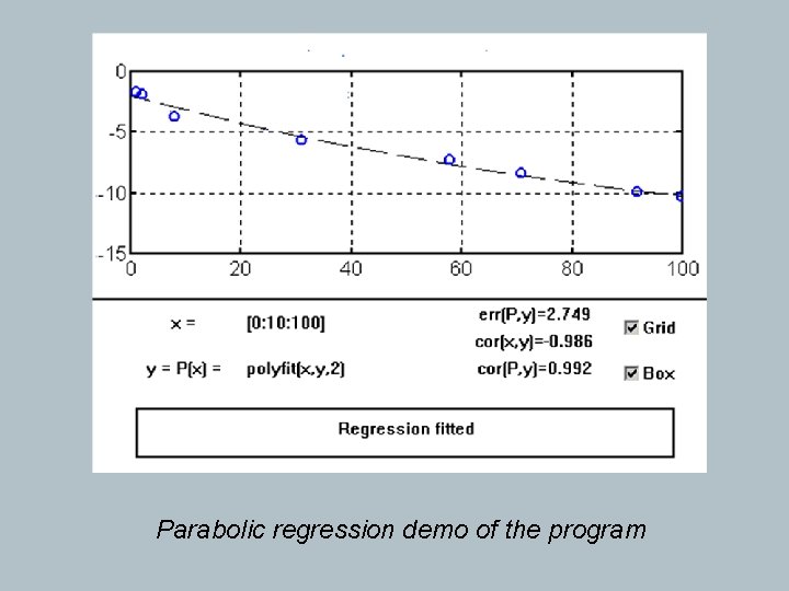
There is an automatic calculus for every defined function the values of the correlation between Ŷ = P(X) and X and the value of residues sum given by the formula: In first figure are presented fitted dates from table with a parabolic regression and program makes the corresponding correlations and sums of residues. In second figure, in same execution, with same dates from table are fitted with a linear regression model and program makes rebuild corresponding correlations and sums of residues.

Linear regression demo of the program

Parabolic regression demo of the program