Numerical Methods Part Simpson Integration Rule For http

Numerical Methods Part: Simpson Integration. Rule For http: //numericalmethods. eng. usf. edu

For more details on this topic Ø Ø Go to http: //numericalmethods. eng. usf. edu Click on Keyword

You are free n n to Share – to copy, distribute, display and perform the work to Remix – to make derivative works

Under the following conditions n n n Attribution — You must attribute the work in the manner specified by the author or licensor (but not in any way that suggests that they endorse you or your use of the work). Noncommercial — You may not use this work for commercial purposes. Share Alike — If you alter, transform, or build upon this work, you may distribute the resulting work only under the same or similar license to this one.

Lecture # 1 Chapter 07. 08: Simpson For Integration. Rule Major: All Engineering Majors Authors: Duc Nguyen http: //numericalmethods. eng. usf. edu Numerical Methods for STEM undergraduates 6/9/2021 http: //numericalmethods. eng. usf. edu 5

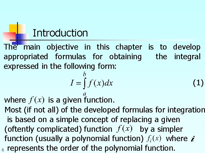
Introduction The main objective in this chapter is to develop appropriated formulas for obtaining the integral expressed in the following form: (1) where is a given function. Most (if not all) of the developed formulas for integration is based on a simple concept of replacing a given (oftently complicated) function by a simpler function (usually a polynomial function) where 6 represents the order of the polynomial function.

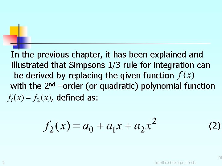
In the previous chapter, it has been explained and illustrated that Simpsons 1/3 rule for integration can be derived by replacing the given function with the 2 nd –order (or quadratic) polynomial function , defined as: (2) 7 lmethods. eng. usf. edu ht

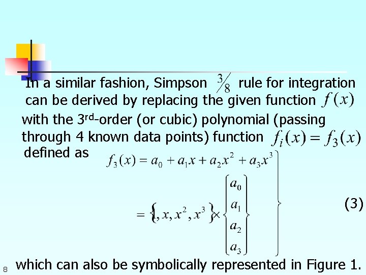
In a similar fashion, Simpson rule for integration can be derived by replacing the given function with the 3 rd-order (or cubic) polynomial (passing through 4 known data points) function defined as (3) 8 which can also be symbolically represented in Figure 1.

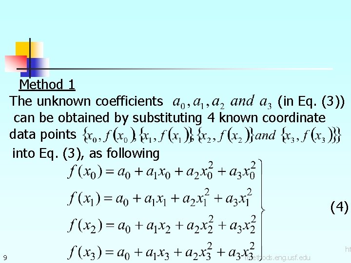
Method 1 The unknown coefficients (in Eq. (3)) can be obtained by substituting 4 known coordinate data points into Eq. (3), as following (4) 9 lmethods. eng. usf. edu ht

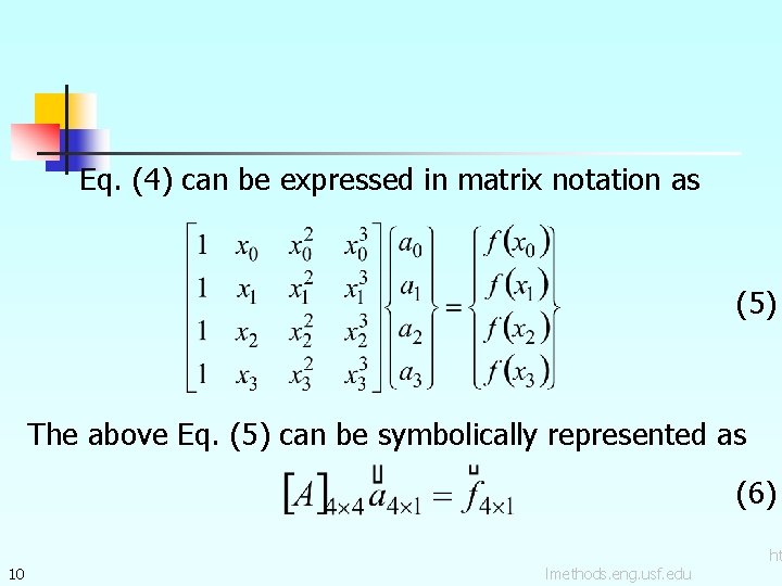
Eq. (4) can be expressed in matrix notation as (5) The above Eq. (5) can be symbolically represented as (6) 10 lmethods. eng. usf. edu ht

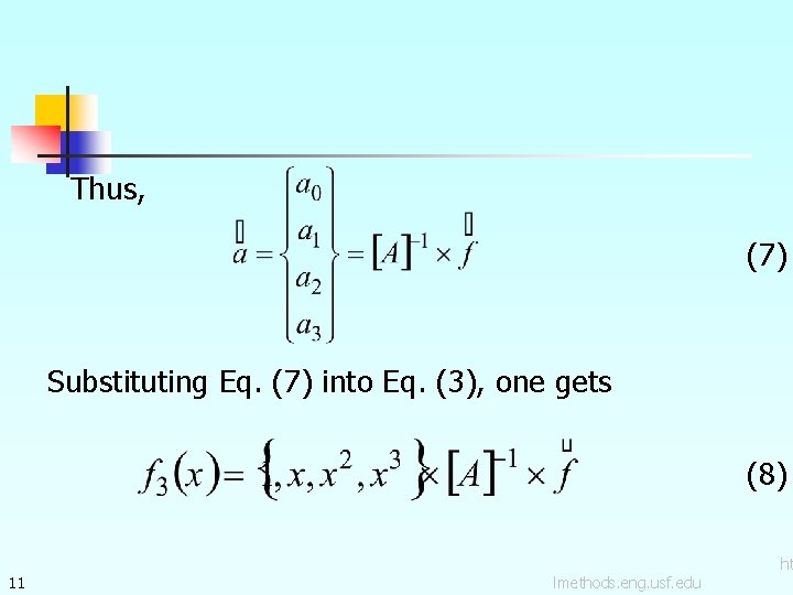
Thus, (7) Substituting Eq. (7) into Eq. (3), one gets (8) 11 lmethods. eng. usf. edu ht

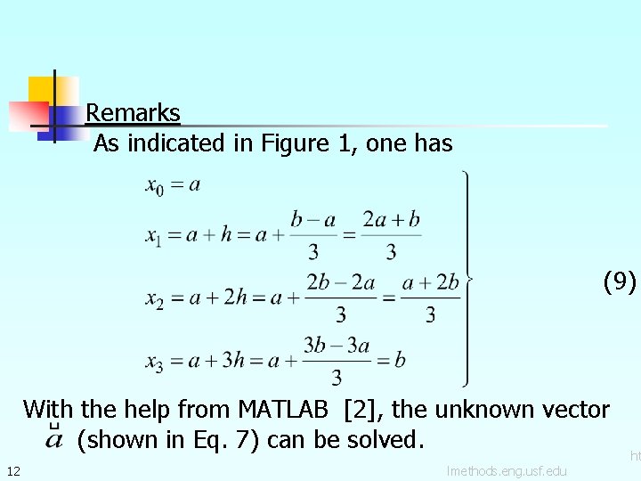
Remarks As indicated in Figure 1, one has (9) With the help from MATLAB [2], the unknown vector (shown in Eq. 7) can be solved. 12 lmethods. eng. usf. edu ht

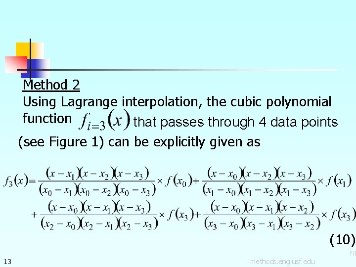
Method 2 Using Lagrange interpolation, the cubic polynomial function that passes through 4 data points (see Figure 1) can be explicitly given as (10) 13 lmethods. eng. usf. edu ht

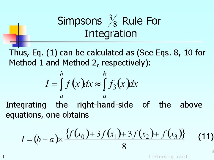
Simpsons Rule For Integration Thus, Eq. (1) can be calculated as (See Eqs. 8, 10 for Method 1 and Method 2, respectively): Integrating the right-hand-side equations, one obtains of the above (11) 14 lmethods. eng. usf. edu ht

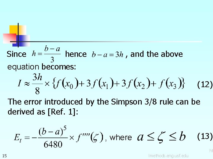
Since hence , and the above equation becomes: (12) The error introduced by the Simpson 3/8 rule can be derived as [Ref. 1]: (13) , where 15 lmethods. eng. usf. edu ht

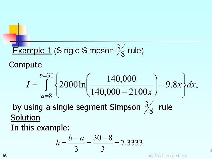
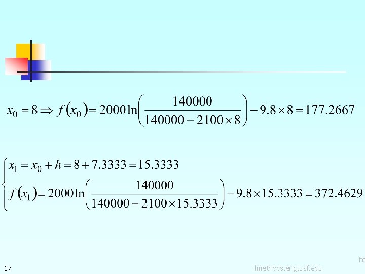
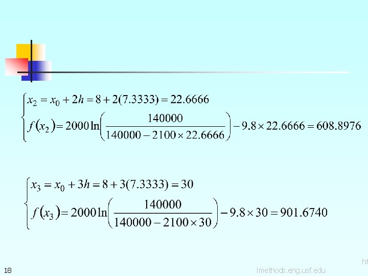
Example 1 (Single Simpson rule) Compute by using a single segment Simpson Solution In this example: 16 rule lmethods. eng. usf. edu ht

17 lmethods. eng. usf. edu ht

18 lmethods. eng. usf. edu ht

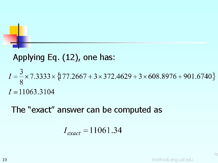
Applying Eq. (12), one has: The “exact” answer can be computed as 19 lmethods. eng. usf. edu ht

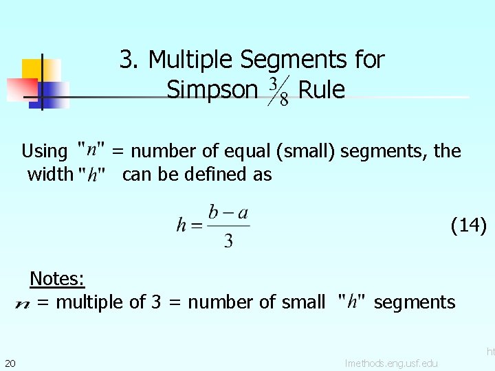
3. Multiple Segments for Simpson Rule Using width = number of equal (small) segments, the can be defined as (14) Notes: = multiple of 3 = number of small 20 segments lmethods. eng. usf. edu ht

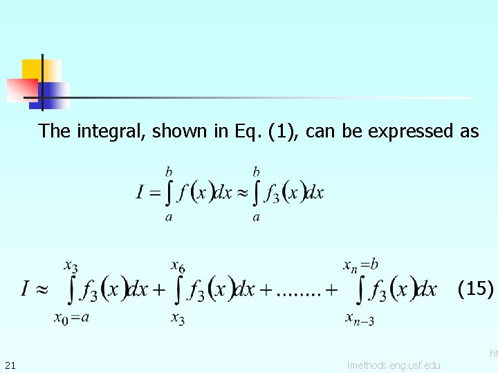
The integral, shown in Eq. (1), can be expressed as (15) 21 lmethods. eng. usf. edu ht

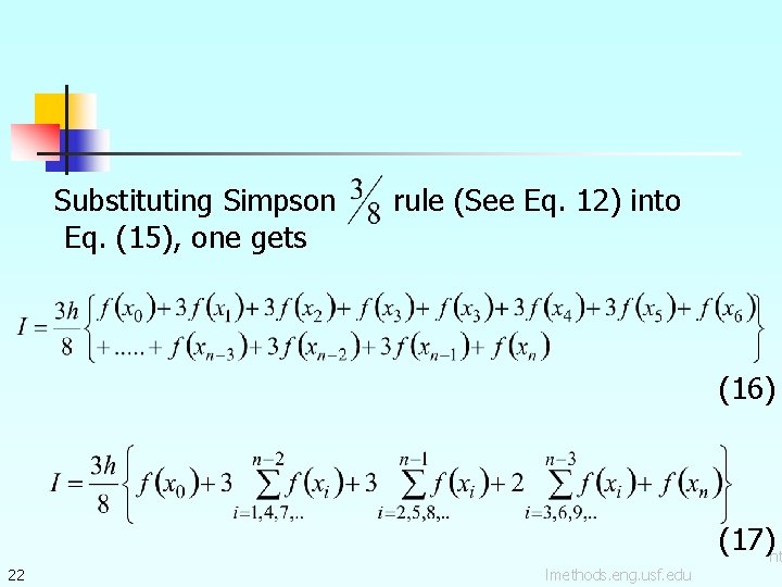
Substituting Simpson Eq. (15), one gets rule (See Eq. 12) into (16) 22 lmethods. eng. usf. edu (17)ht

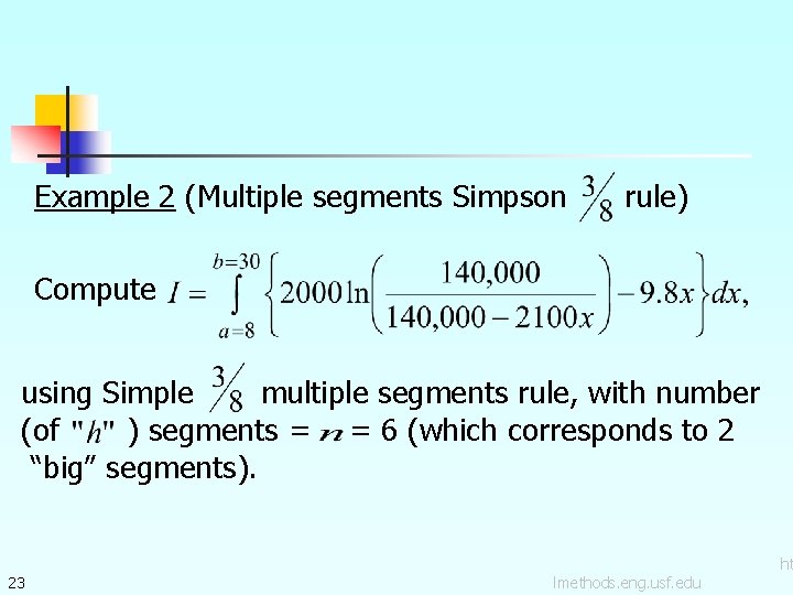
Example 2 (Multiple segments Simpson rule) Compute using Simple multiple segments rule, with number (of ) segments = = 6 (which corresponds to 2 “big” segments). 23 lmethods. eng. usf. edu ht

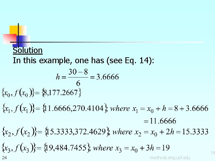
Solution In this example, one has (see Eq. 14): 24 lmethods. eng. usf. edu ht

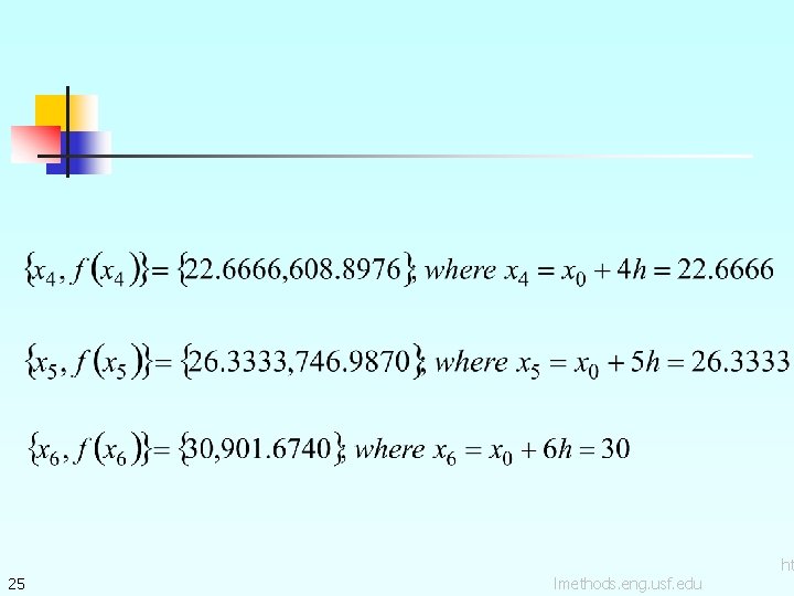
25 lmethods. eng. usf. edu ht

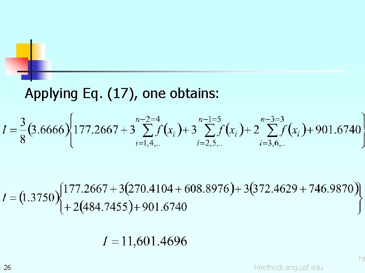
Applying Eq. (17), one obtains: 26 lmethods. eng. usf. edu ht

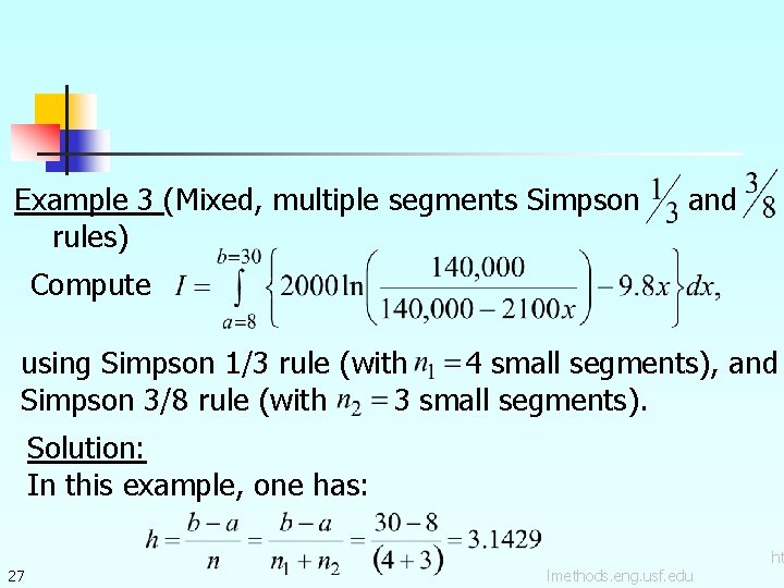
Example 3 (Mixed, multiple segments Simpson rules) and Compute using Simpson 1/3 rule (with 4 small segments), and Simpson 3/8 rule (with 3 small segments). Solution: In this example, one has: 27 lmethods. eng. usf. edu ht

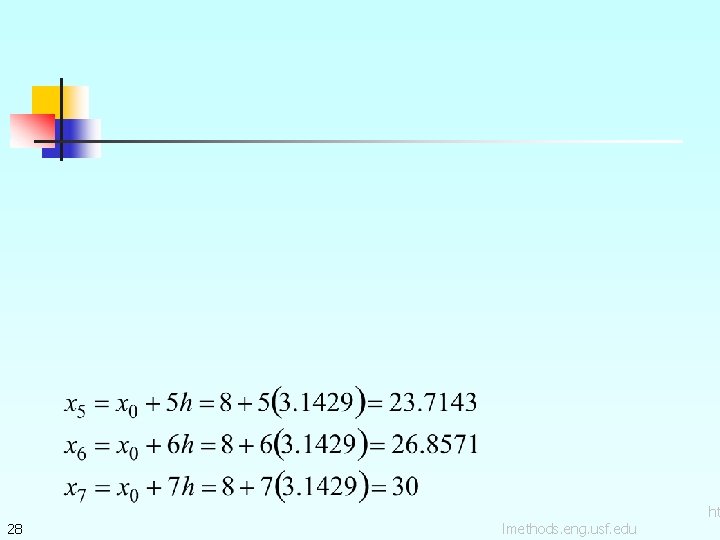
28 lmethods. eng. usf. edu ht

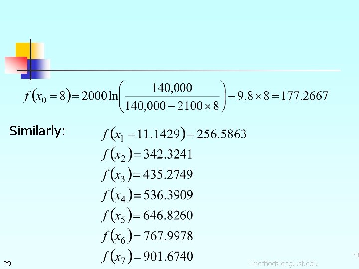
Similarly: 29 lmethods. eng. usf. edu ht

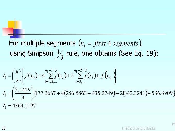
For multiple segments using Simpson rule, one obtains (See Eq. 19): 30 lmethods. eng. usf. edu ht

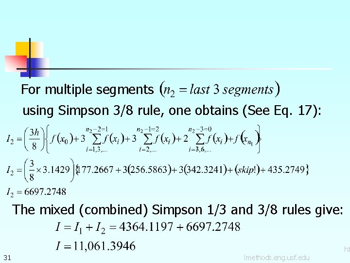
For multiple segments using Simpson 3/8 rule, one obtains (See Eq. 17): The mixed (combined) Simpson 1/3 and 3/8 rules give: 31 lmethods. eng. usf. edu ht

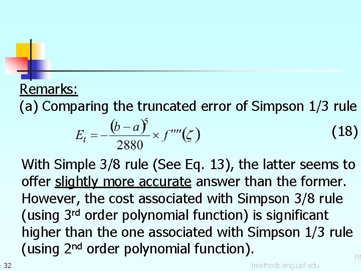
Remarks: (a) Comparing the truncated error of Simpson 1/3 rule (18) 32 With Simple 3/8 rule (See Eq. 13), the latter seems to offer slightly more accurate answer than the former. However, the cost associated with Simpson 3/8 rule (using 3 rd order polynomial function) is significant higher than the one associated with Simpson 1/3 rule (using 2 nd order polynomial function). ht lmethods. eng. usf. edu

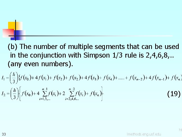
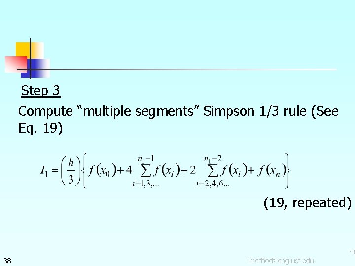
(b) The number of multiple segments that can be used in the conjunction with Simpson 1/3 rule is 2, 4, 6, 8, . . (any even numbers). (19) 33 lmethods. eng. usf. edu ht

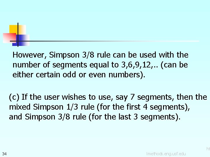
However, Simpson 3/8 rule can be used with the number of segments equal to 3, 6, 9, 12, . . (can be either certain odd or even numbers). (c) If the user wishes to use, say 7 segments, then the mixed Simpson 1/3 rule (for the first 4 segments), and Simpson 3/8 rule (for the last 3 segments). 34 lmethods. eng. usf. edu ht

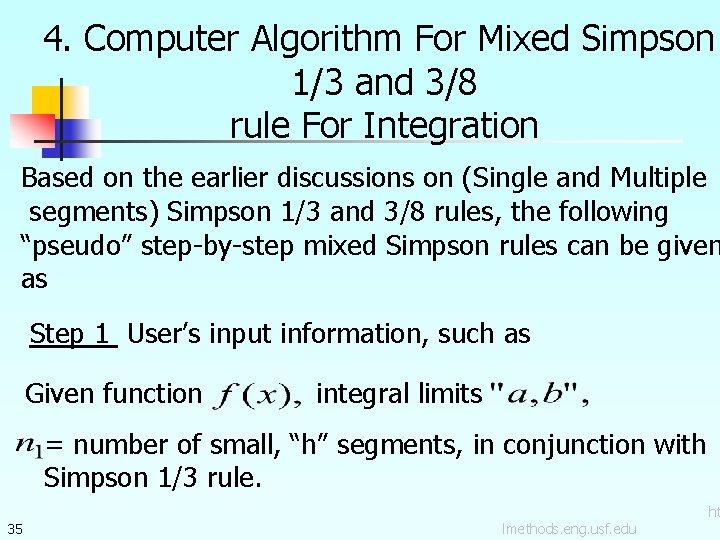
4. Computer Algorithm For Mixed Simpson 1/3 and 3/8 rule For Integration Based on the earlier discussions on (Single and Multiple segments) Simpson 1/3 and 3/8 rules, the following “pseudo” step-by-step mixed Simpson rules can be given as Step 1 User’s input information, such as Given function integral limits = number of small, “h” segments, in conjunction with Simpson 1/3 rule. 35 lmethods. eng. usf. edu ht

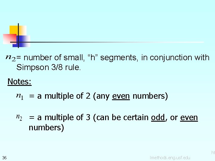
= number of small, “h” segments, in conjunction with Simpson 3/8 rule. Notes: = a multiple of 2 (any even numbers) = a multiple of 3 (can be certain odd, or even numbers) 36 lmethods. eng. usf. edu ht

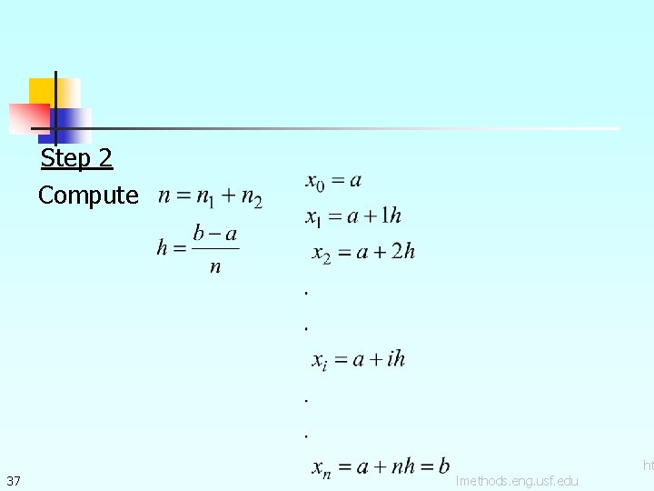
Step 2 Compute 37 lmethods. eng. usf. edu ht

Step 3 Compute “multiple segments” Simpson 1/3 rule (See Eq. 19) (19, repeated) 38 lmethods. eng. usf. edu ht

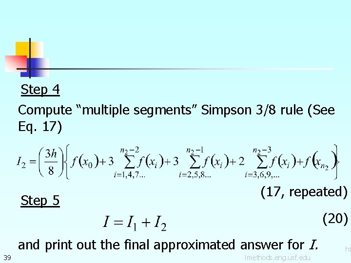
Step 4 Compute “multiple segments” Simpson 3/8 rule (See Eq. 17) Step 5 (17, repeated) (20) and print out the final approximated answer for I. 39 lmethods. eng. usf. edu ht

THE END http: //numericalmethods. eng. usf. edu

Acknowledgement This instructional power point brought to you by Numerical Methods for STEM undergraduate http: //numericalmethods. eng. usf. edu Committed to bringing numerical methods to the undergraduate

For instructional videos on other topics, go to http: //numericalmethods. eng. usf. edu/videos/ This material is based upon work supported by the National Science Foundation under Grant # 0717624. Any opinions, findings, and conclusions or recommendations expressed in this material are those of the author(s) and do not necessarily reflect the views of the National Science Foundation.

The End - Really