Numerical Methods Marisa Villano Tom Fagan Dave Fairburn

Numerical Methods Marisa Villano, Tom Fagan, Dave Fairburn, Chris Savino, David Goldberg, Daniel Rave

An Overview The Method of Finite Differences n Error Approximations and Dangers n Approxmations to Diffusions n Crank Nicholson Scheme n Stability Criterion n

Finite Differences Best known numerical method of approximation Marisa Villano

Finite Differences n Approximating the derivative with a difference quotient from the Taylor series n Function of One Variable Choose mesh size Δx n Then uj ~ u(jΔx) n
 / Δx n Forward difference:")
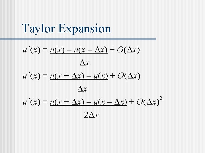
First Derivative Approximations n Backward difference: (uj – uj-1) / Δx n Forward difference: (uj+1 – uj) / Δx n Centered difference: (uj+1 – uj-1) / 2Δx
 = u(x) + u΄(x)Δx + 1/2")
Taylor Expansion n n 2 u(x + Δx) = u(x) + u΄(x)Δx + 1/2 u˝(x)(Δx) 3 4 + 1/6 u˝΄(x)(Δx) + O(Δx) u(x – Δx) = u(x) – u΄(x)Δx + 1/2 u˝(x)(Δx) 3 4 - 1/6 u˝΄(x)(Δx) + O(Δx) 2
 / (Δx)")
Second Derivative Approximation n Centered difference: (uj+1 – 2 uj + uj-1) / (Δx) n Taylor Expansion 2 u˝(x) = u(x + Δx) – 2 u(x) + u(x – Δx) + O(Δx) 2
 ~ uj n Backward difference for t")
Function of Two Variables n u(jΔx, nΔt) ~ uj n Backward difference for t and x ∂u (jΔx, nΔt) ~ (ujn – ujn-1) / Δt ∂t ∂u (jΔx, nΔt) ~ (ujn – ujn-1) / Δx ∂x
")
Function of Two Variables n Forward difference for t and x ∂u (jΔx, nΔt) ~ (ujn+1 – ujn ) / Δt ∂t ∂u (jΔx, nΔt) ~ (ujn+1 – ujn ) / Δx ∂x
")
Function of Two Variables n Centered difference for t and x ∂u (jΔx, nΔt) ~ (ujn+1 – ujn-1) / (2Δt) ∂t ∂u (jΔx, nΔt) ~ (ujn+1 – ujn-1) / (2Δx) ∂x

Error n Truncation Error: introduced in the solution by the approximation of the derivative n Local Error: from each term of the equation n Global error n Error: from the accumulation of local Roundoff Error: introduced in the computation by the finite number of digits used by the computer

The Dangers of the Finite Difference Method Evidence from an example in 8. 1 Dave Fairburn
 = h(x) n We")
Example from 8. 1 Consider ut = uxx u(x, 0) = h(x) n We will use the finite difference method to approximate the solution n Forward difference for ut n Centered difference for uxx n Re-write equation in terms of the finite difference approximations n

Finite Difference Eqn. n ujn+1 - ujn = unj+1 - 2 ujn + unj-1 t ( x) 2 Error: The local truncation error is O( t) from the left hand side and is O( x)2 from the right hand side.

Assumptions Assume that we choose a small change in x, and that the denominator on both sides of the equation are equal. n We are now left with the scheme: ujn+1 = unj+1 - unj + unj-1 n Solving u with this scheme is now easy to do once we have the initial data. n
 = h(x) = a step function with the following")
Initial Data Let u(x, 0) = h(x) = a step function with the following properties: h(x) = 0 for all j except for j = 5, so hj = 0 0 1 0 0 0 …. n Initially, only a certain section, which is at j = 5 is equal to the value of 1. n “j” serves as the counter for the x values. n

How to solve? n n n We know u 0 j = 1 at j = 5 and 0 at all other j initially (given by superscript 0). We can plug into our scheme to solve for u 1 j at all j’s. u 1 j = u 0 j-1 - u 0 j + u 0 j+1 u 15 = -1; u 14 = 1; u 16 = 1 Now we can continue to increase the # of iterations, n, and create a table…

Solution for 4 iterations n v a l u e s 4 1 -4 10 -16 19 -16 10 -4 1 0 3 0 1 -3 6 -7 6 -3 1 0 0 2 0 0 1 -2 3 -2 1 0 0 0 1 -1 1 0 0 0 0 0 1 2 3 4 5 6 7 8 9 10 j values

Analysis of Solution n n Is this solution viable? Maximum principle states that the solution must be between 0 and 1 given our initial data At n = 4, our solution has already ballooned to u = 19! Clearly, there are cases when the finite difference method can pose serious problems.

Charting the Error n Assume the solution is constant and equal to 0. 5 (halfway between the possible 0 and 1)

Lessons Learned While the finite difference method is easy and convenient to use in many cases, there are some dangers associated with the method. n We will investigate why the assumption that allowed us to simplify the scheme could have been a major contributor to the large error. n

Approximations of Diffusions Neumann Boundary Conditions and the Crank-Nicolson Scheme Chris Savino

Approximations of Diffusions n n n Errors have accumulated from the approximations of the derivatives using the previous scheme The problem is the choice of the mesh Δt to the mesh Δx Let s= can solve scheme

Neumann Boundary Conditions n 0 x l n Simplest Approximations are

n To get smallest error, we use centered differences for the derivatives on the boundary Introduce ghost points n Boundary Conditions become n

Crank-Nicolson Scheme Can avoid any restrictions on stability conditions n Unconditionally stable no matter what the value of s is. n

n Centered Second Difference: n Pick a number theta between 0 and 1 Theta scheme: n

n We analyze the scheme by plugging in a separated solution n Therefore

n Must Check stability condition n If n Therefore then is always true

n n If then there is no restriction on the size of s for stability to hold The scheme is unconditionally stable When theta = ½ it is called the Crank-Nicolson scheme If theta < ½ then the scheme is stable if

Stability Criterion Approximations of the diffusion equation, ut=uxx David Goldberg

Stability Criterion The method of finite differences gives an answer, but it does not guarantee that this answer is meaningful. n Values must be chosen appropriately, to ensure that the results make sense and are applicable to real world scenarios. n This condition, that values must satisfy in order to be worthwhile, is called the “stability criterion. ” n

Example n As per the book, take, for instance, the diffusion problem:
 looks")
Example, continued 1. 8 As can be easily shown, the graph of φ(x) looks like this. 1. 6 1. 4 1. 2 1 0. 8 0. 6 0. 4 0. 2 0 0 0. 5 1 1. 5 2 2. 5 3 3. 5

Example, continued In attempting to use the method of finite differences, we are using a forward difference for ut and a centered difference for uxx. n This means that n n It is important to note here that the superscript n denotes a counter on the t variable, and the subscript j denotes a counter on the x variable.

Example, continued n In order to make the calculations a bit cleaner, we are introducing a variable, s, which is defined by n Rearranging, we have n It would be nice if we could just plug in values and get a valid result…

Example, continued n n 2 However, putting in different values can lead to the results being close to, or far from, that actual answer. For instance, letting ∆x=π/20, and letting s=5/11, we get a relatively nice result. Letting s=5/9 does not get such a nice result. 2 1. 5 1 1 0. 5 0 0 0 n 1 2 3 4 0 1 So what, of significance, changes? 2 3 4

Example, Continued n As it turns out, changing the value of s can significantly change the validity of the solution. To see why, we return to our equation.

Example, continued n Since the left hand side is a function of T and the right hand side is a function of X, they must be equal to a constant.

Example, continued n This is a discrete version of an ODE, which when solved gives

Example, finished Thus, to achieve stability, . This is why setting s=5/9 didn’t give a valid result. n It is to be noted that usually the necessary criterion is that , but that in this case it was irrelevant. n So the stability criterion must be worked out before one can effectively use the method of finite differences. n

Approximations of Diffusions Example from 8. 2 Daniel Rave

Summary n Breif Review of Methods n Wide Applicability n Importance of Stability
- Slides: 44