Numerical Methods and Software for Partial Differential Equations

Numerical Methods and Software for Partial Differential Equations Lecturer: Dr Yvonne Fryer Time: Mondays 10 am-1 pm Location: QA 210 / KW 116 (Black) 1

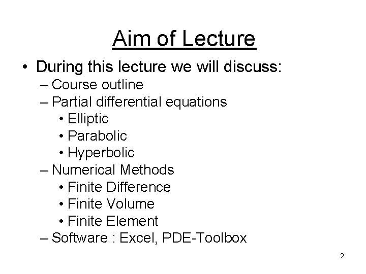
Aim of Lecture • During this lecture we will discuss: – Course outline – Partial differential equations • Elliptic • Parabolic • Hyperbolic – Numerical Methods • Finite Difference • Finite Volume • Finite Element – Software : Excel, PDE-Toolbox 2

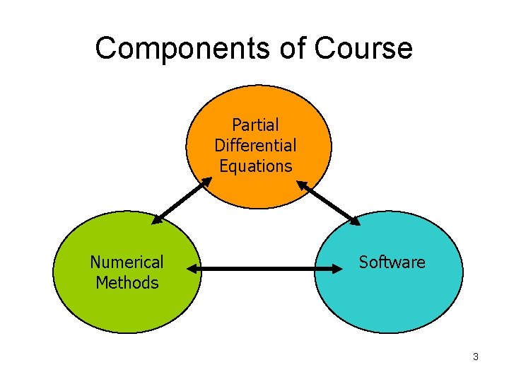
Components of Course Partial Differential Equations Numerical Methods Software 3

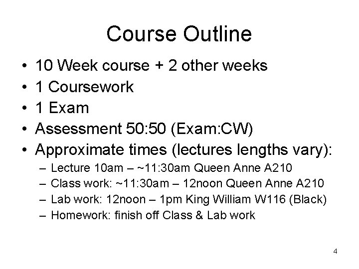
Course Outline • • • 10 Week course + 2 other weeks 1 Coursework 1 Exam Assessment 50: 50 (Exam: CW) Approximate times (lectures lengths vary): – – Lecture 10 am – ~11: 30 am Queen Anne A 210 Class work: ~11: 30 am – 12 noon Queen Anne A 210 Lab work: 12 noon – 1 pm King William W 116 (Black) Homework: finish off Class & Lab work 4

Textbooks • Morton & Mayers, Numerical Solution of Partial Differential Equations (Cambridge University Press, 2005) is recommended if you want to do some background reading • Burden & Faires, Numerical Analysis (Brooks Cole, 2001) has a good chapter on Numerical Methods for PDEs • However you do not require either of these books – the lecture notes should suffice 5

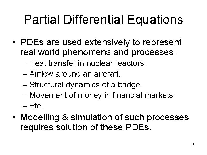
Partial Differential Equations • PDEs are used extensively to represent real world phenomena and processes. – Heat transfer in nuclear reactors. – Airflow around an aircraft. – Structural dynamics of a bridge. – Movement of money in financial markets. – Etc. • Modelling & simulation of such processes requires solution of these PDEs. 6

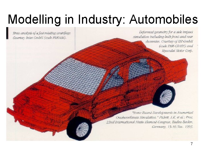
Modelling in Industry: Automobiles 7

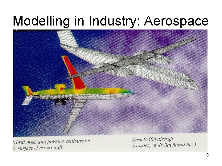
Modelling in Industry: Aerospace 8

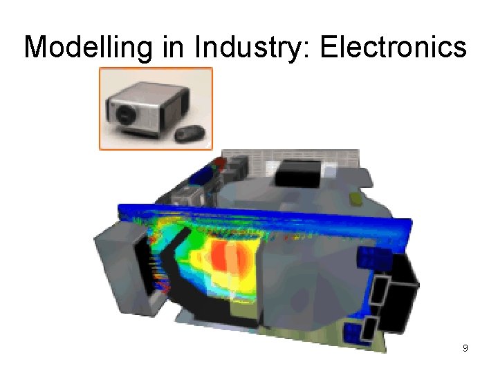
Modelling in Industry: Electronics 9

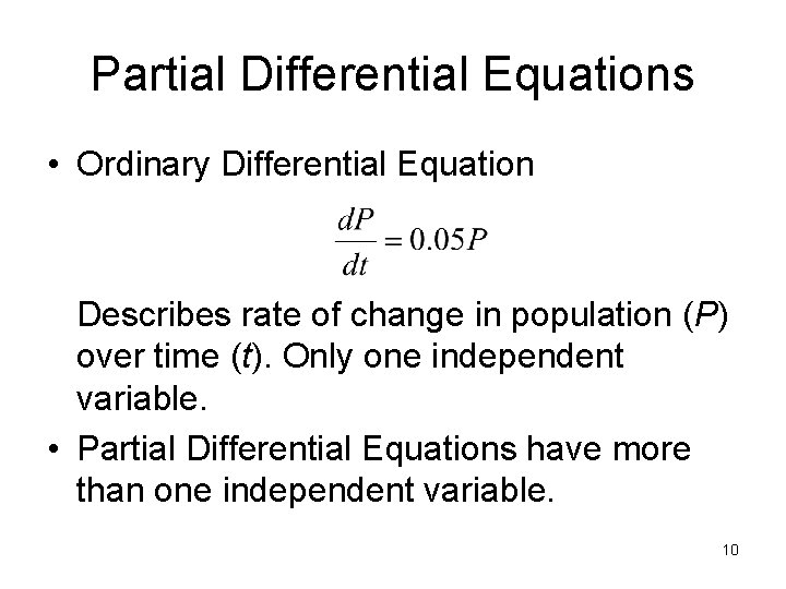
Partial Differential Equations • Ordinary Differential Equation Describes rate of change in population (P) over time (t). Only one independent variable. • Partial Differential Equations have more than one independent variable. 10

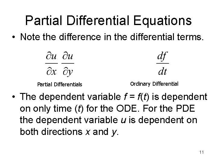
Partial Differential Equations • Note the difference in the differential terms. Partial Differentials Ordinary Differential • The dependent variable f = f(t) is dependent on only time (t) for the ODE. For the PDE the dependent variable u is dependent on both directions x and y. 11

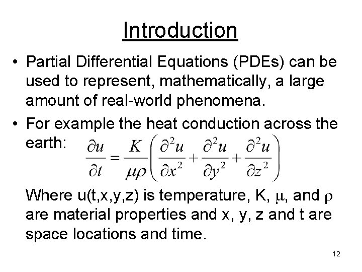
Introduction • Partial Differential Equations (PDEs) can be used to represent, mathematically, a large amount of real-world phenomena. • For example the heat conduction across the earth: Where u(t, x, y, z) is temperature, K, , and are material properties and x, y, z and t are space locations and time. 12

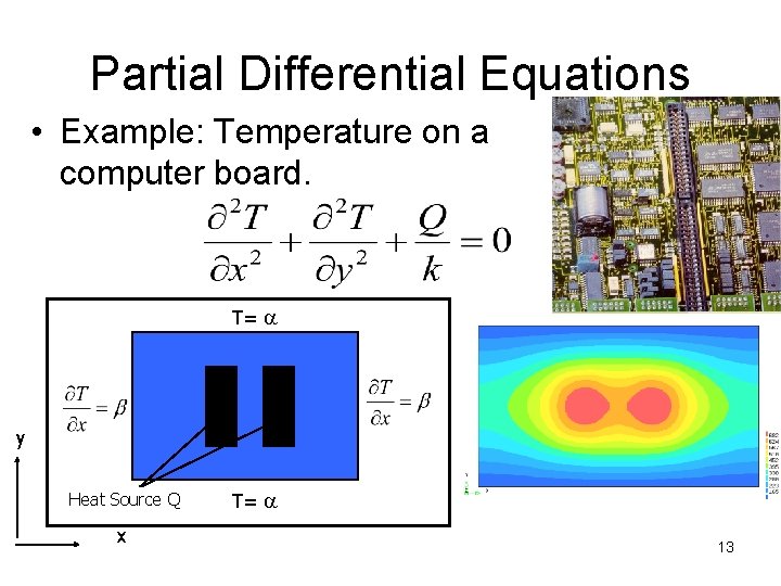
Partial Differential Equations • Example: Temperature on a computer board. T= y Heat Source Q x T= 13

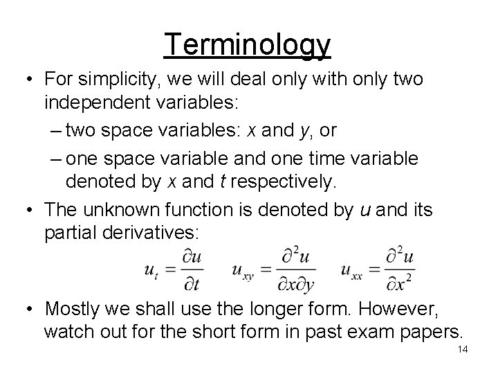
Terminology • For simplicity, we will deal only with only two independent variables: – two space variables: x and y, or – one space variable and one time variable denoted by x and t respectively. • The unknown function is denoted by u and its partial derivatives: • Mostly we shall use the longer form. However, watch out for the short form in past exam papers. 14

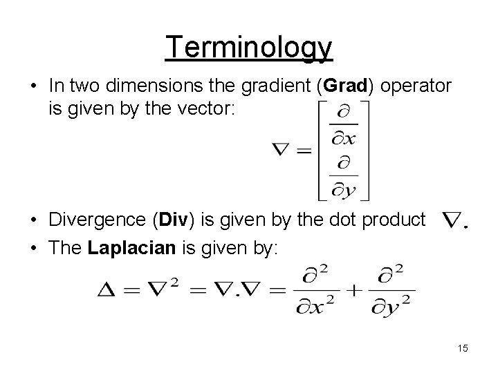
Terminology • In two dimensions the gradient (Grad) operator is given by the vector: • Divergence (Div) is given by the dot product • The Laplacian is given by: 15

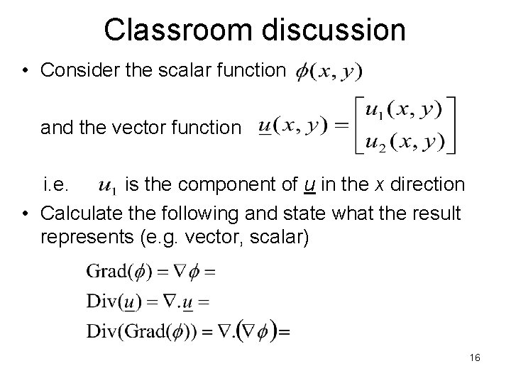
Classroom discussion • Consider the scalar function and the vector function i. e. is the component of u in the x direction • Calculate the following and state what the result represents (e. g. vector, scalar) 16

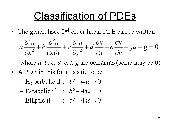
Classification of PDEs • The generalised 2 nd order linear PDE can be written: where a, b, c, d, e, f, g are constants (some may be 0). • A PDE in this form is said to be: – Hyperbolic if : b 2 – 4 ac > 0 – Parabolic if : b 2 – 4 ac = 0 – Elliptic if : b 2 – 4 ac < 0 17

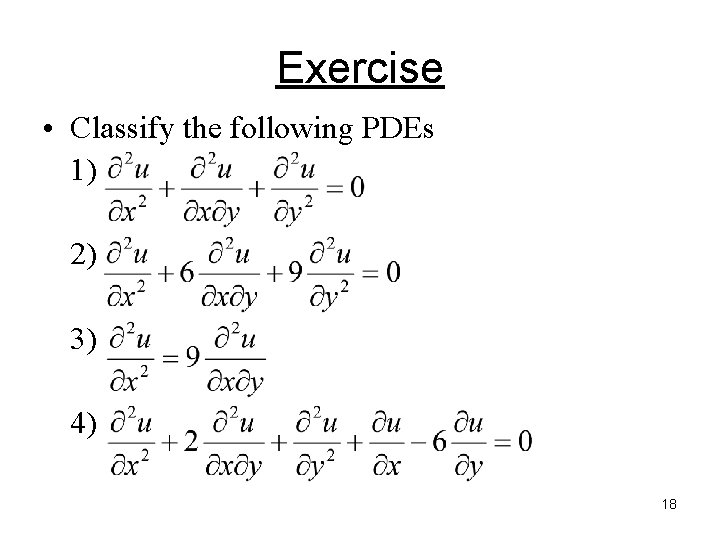
Exercise • Classify the following PDEs 1) 2) 3) 4) 18

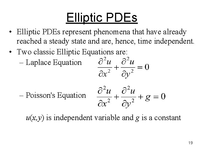
Elliptic PDEs • Elliptic PDEs represent phenomena that have already reached a steady state and are, hence, time independent. • Two classic Elliptic Equations are: – Laplace Equation – Poisson's Equation u(x, y) is independent variable and g is a constant 19

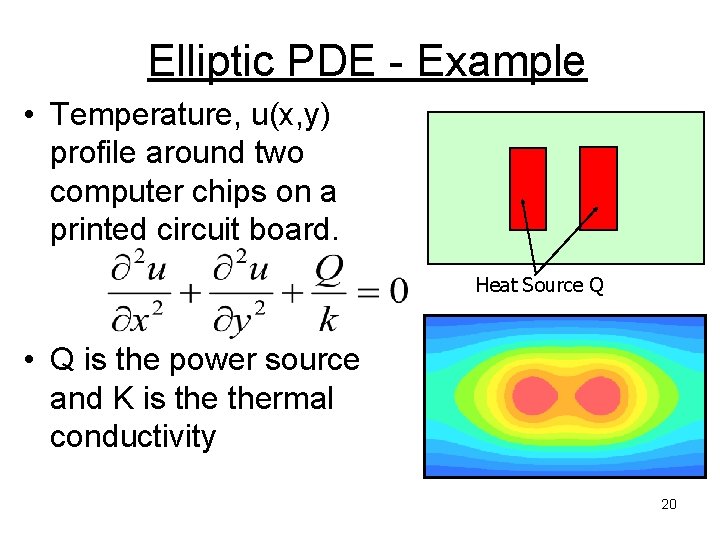
Elliptic PDE - Example • Temperature, u(x, y) profile around two computer chips on a printed circuit board. Heat Source Q • Q is the power source and K is thermal conductivity 20

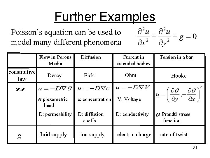
Further Examples Poisson’s equation can be used to model many different phenomena Flow in Porous Media constitutive law g Darcy Diffusion Fick : piezometric head c: concentration D: permeability D: diffusion coeffs fluid supply ion supply Current in extended bodies Ohm Torsion in a bar Hooke V: Voltage D: conductivity : Prandtl stress function electric charge rate of twist 21

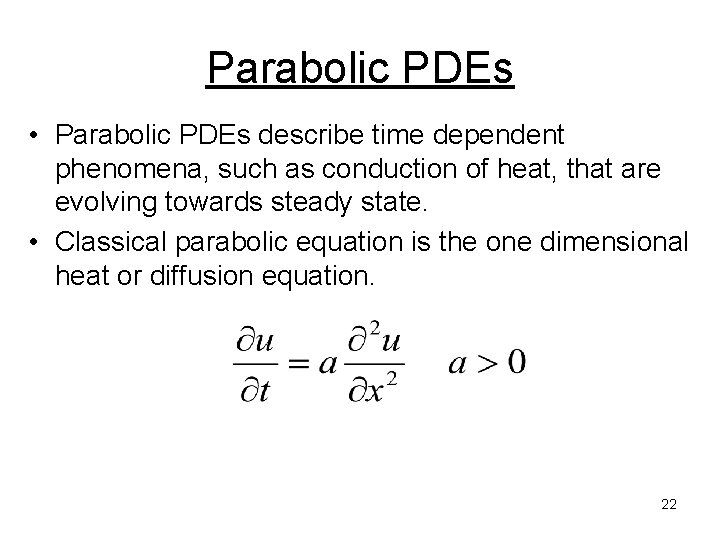
Parabolic PDEs • Parabolic PDEs describe time dependent phenomena, such as conduction of heat, that are evolving towards steady state. • Classical parabolic equation is the one dimensional heat or diffusion equation. 22

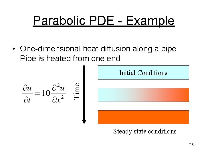
Parabolic PDE - Example • One-dimensional heat diffusion along a pipe. Pipe is heated from one end. Time Initial Conditions Steady state conditions 23

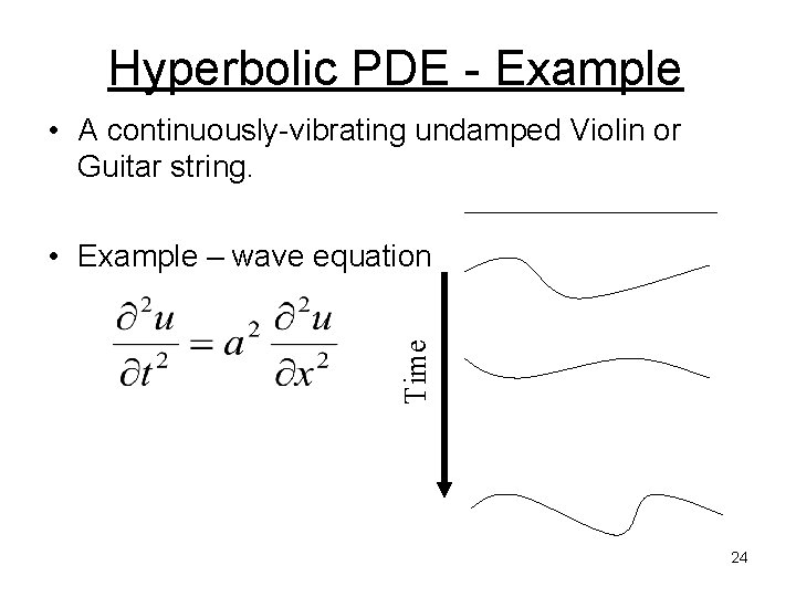
Hyperbolic PDE - Example • A continuously-vibrating undamped Violin or Guitar string. Time • Example – wave equation 24

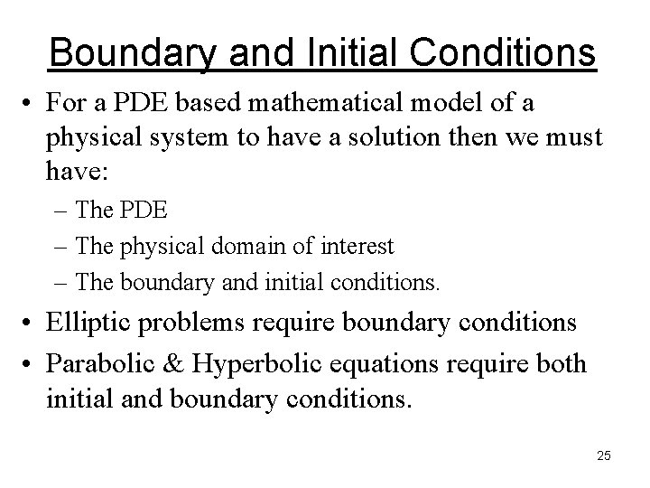
Boundary and Initial Conditions • For a PDE based mathematical model of a physical system to have a solution then we must have: – The PDE – The physical domain of interest – The boundary and initial conditions. • Elliptic problems require boundary conditions • Parabolic & Hyperbolic equations require both initial and boundary conditions. 25

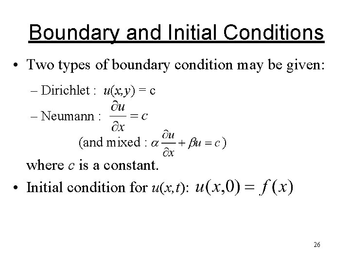
Boundary and Initial Conditions • Two types of boundary condition may be given: – Dirichlet : u(x, y) = c – Neumann : (and mixed : ) where c is a constant. • Initial condition for u(x, t): 26

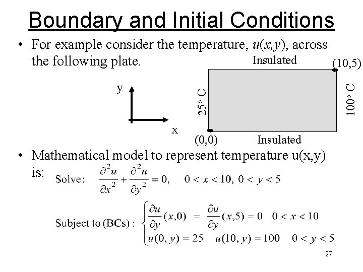
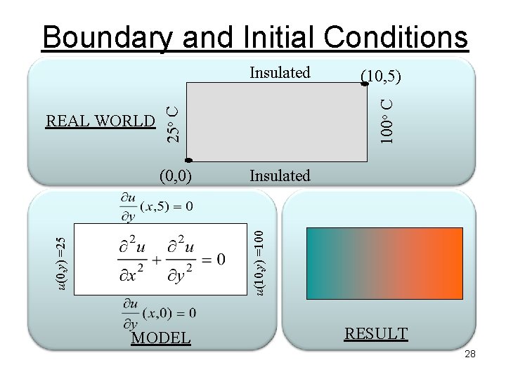
Boundary and Initial Conditions 25 o C y 100 o C • For example consider the temperature, u(x, y), across Insulated the following plate. (10, 5) x (0, 0) Insulated • Mathematical model to represent temperature u(x, y) is: 27

Boundary and Initial Conditions 25 o C REAL WORLD Insulated u(0, y) =25 u(10, y) =100 (0, 0) (10, 5) 100 o C Insulated MODEL RESULT 28

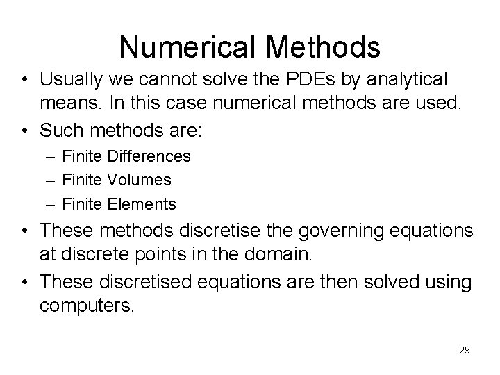
Numerical Methods • Usually we cannot solve the PDEs by analytical means. In this case numerical methods are used. • Such methods are: – Finite Differences – Finite Volumes – Finite Elements • These methods discretise the governing equations at discrete points in the domain. • These discretised equations are then solved using computers. 29

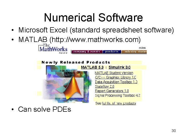
Numerical Software • Microsoft Excel (standard spreadsheet software) • MATLAB (http: //www. mathworks. com) • Can solve PDEs 30

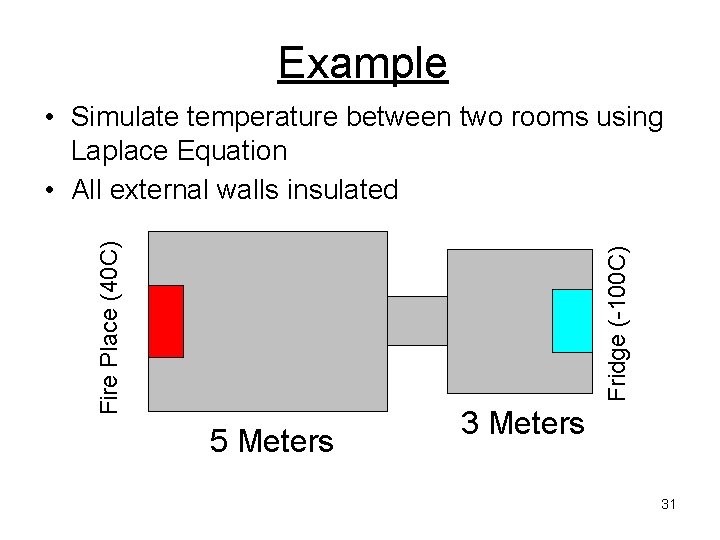
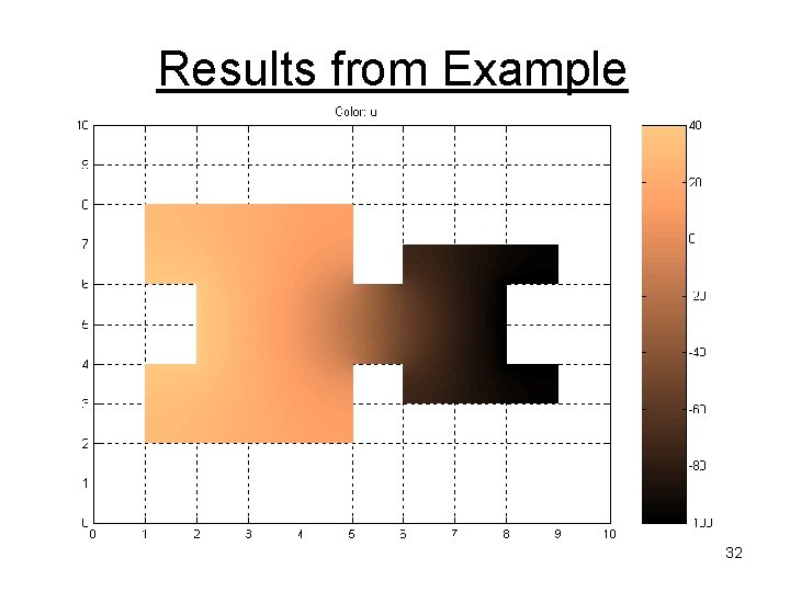
Example Fridge (-100 C) Fire Place (40 C) • Simulate temperature between two rooms using Laplace Equation • All external walls insulated 5 Meters 31

Results from Example 32