Numerical descriptions of distributions Describe the shape center

Numerical descriptions of distributions Describe the shape, center, and spread of a distribution… for shape, see slide #6 below. . . Center: mean and median Spread: range, IQR, standard deviation We treat these as aids to understanding the distribution of the variable at hand… The mean is often called the "average" and is in fact the arithmetic average ("add all the values and divide by the number of observations").

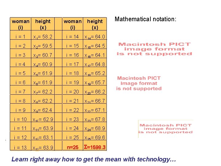
woman (i) height (x) i=1 x 1= 58. 2 i = 14 x 14= 64. 0 i=2 x 2= 59. 5 i = 15 x 15= 64. 5 i=3 x 3= 60. 7 i = 16 x 16= 64. 1 i=4 x 4= 60. 9 i = 17 x 17= 64. 8 i=5 x 5= 61. 9 i = 18 x 18= 65. 2 i=6 x 6= 61. 9 i = 19 x 19= 65. 7 i=7 x 7= 62. 2 i = 20 x 20= 66. 2 i=8 x 8= 62. 2 i = 21 x 21= 66. 7 i=9 x 9= 62. 4 i = 22 x 22= 67. 1 i = 10 x 10= 62. 9 i = 23 x 23= 67. 8 i = 11 x 11= 63. 9 i = 24 x 24= 68. 9 i = 12 x 12= 63. 1 i = 25 x 25= 69. 6 i = 13 x 13= 63. 9 n=25 S=1598. 3 Mathematical notation: Learn right away how to get the mean with technology…

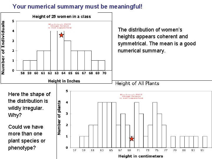
Your numerical summary must be meaningful! Height of 25 women in a class The distribution of women’s heights appears coherent and symmetrical. The mean is a good numerical summary. Here the shape of the distribution is wildly irregular. Why? Could we have more than one plant species or phenotype?

58 60 62 64 66 68 70 72 74 76 78 80 82 A single numerical summary here would not make sense. 84

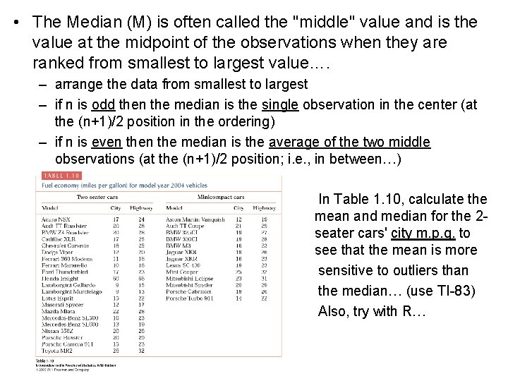
• The Median (M) is often called the "middle" value and is the value at the midpoint of the observations when they are ranked from smallest to largest value…. – arrange the data from smallest to largest – if n is odd then the median is the single observation in the center (at the (n+1)/2 position in the ordering) – if n is even the median is the average of the two middle observations (at the (n+1)/2 position; i. e. , in between…) In Table 1. 10, calculate the mean and median for the 2 seater cars' city m. p. g. to see that the mean is more sensitive to outliers than the median… (use TI-83) Also, try with R…

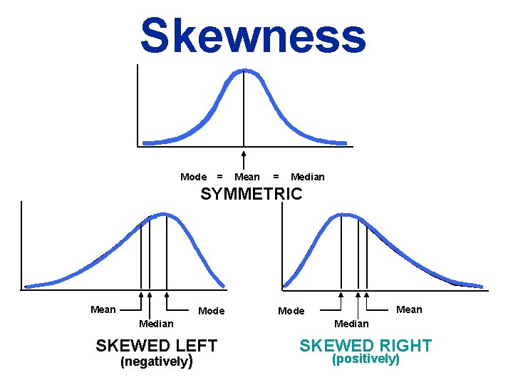
Skewness Mode = Mean = Median SYMMETRIC Mean Mode Median SKEWED LEFT (negatively) Mean Mode Median SKEWED RIGHT (positively)

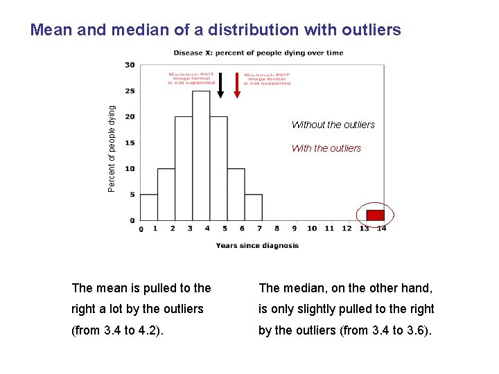
Percent of people dying Mean and median of a distribution with outliers Without the outliers With the outliers The mean is pulled to the The median, on the other hand, right a lot by the outliers is only slightly pulled to the right (from 3. 4 to 4. 2). by the outliers (from 3. 4 to 3. 6).

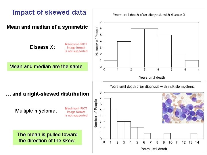
Impact of skewed data Mean and median of a symmetric Disease X: Mean and median are the same. … and a right-skewed distribution Multiple myeloma: The mean is pulled toward the direction of the skew.

Spread: percentiles, quartiles (Q 1 and Q 3), IQR, 5 -number summary (and boxplots), range, standard deviation pth percentile of a variable is a data value such that p% of the values of the variable are less than or equal to it. the lower (Q 1) and upper (Q 3) quartiles are special percentiles dividing the data into quarters (fourths). get them by finding the medians of the lower and upper halfs of the data IQR = interquartile range = Q 3 - Q 1 = spread of the middle 50% of the data. IQR is used with the socalled 1. 5*IQR criterion for outliers - know this!

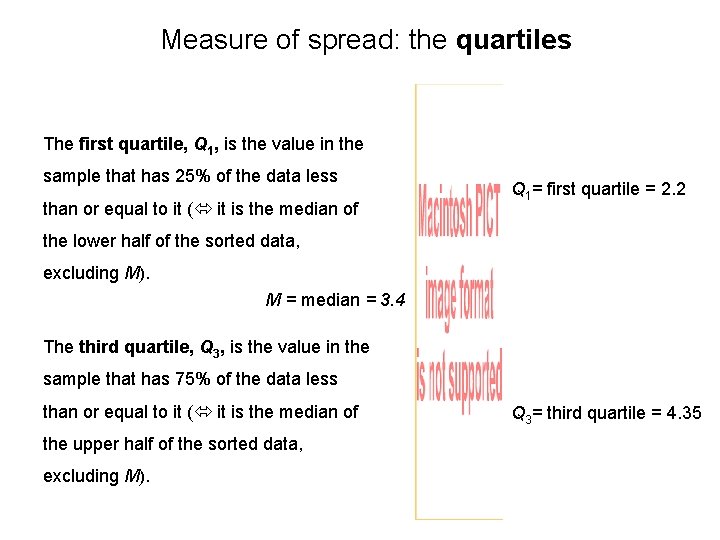
Measure of spread: the quartiles The first quartile, Q 1, is the value in the sample that has 25% of the data less than or equal to it ( it is the median of Q 1= first quartile = 2. 2 the lower half of the sorted data, excluding M). M = median = 3. 4 The third quartile, Q 3, is the value in the sample that has 75% of the data less than or equal to it ( it is the median of the upper half of the sorted data, excluding M). Q 3= third quartile = 4. 35

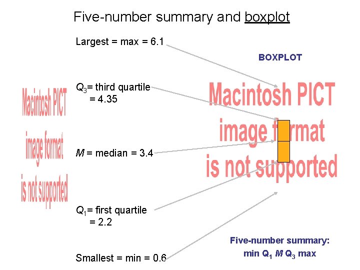
Five-number summary and boxplot Largest = max = 6. 1 BOXPLOT Q 3= third quartile = 4. 35 M = median = 3. 4 Q 1= first quartile = 2. 2 Smallest = min = 0. 6 Five-number summary: min Q 1 M Q 3 max

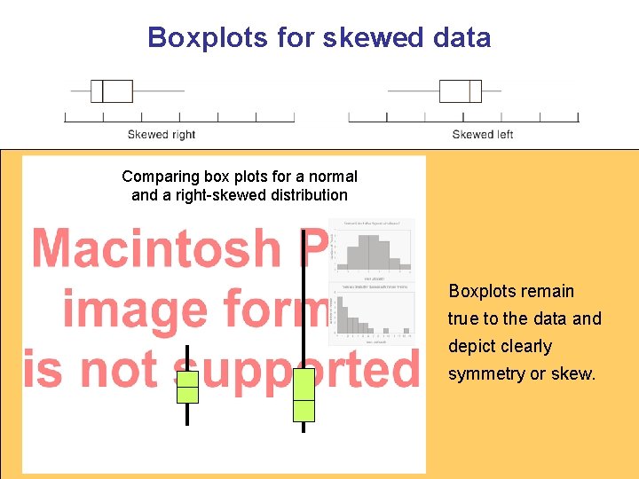
Boxplots for skewed data Comparing box plots for a normal and a right-skewed distribution Boxplots remain true to the data and depict clearly symmetry or skew.

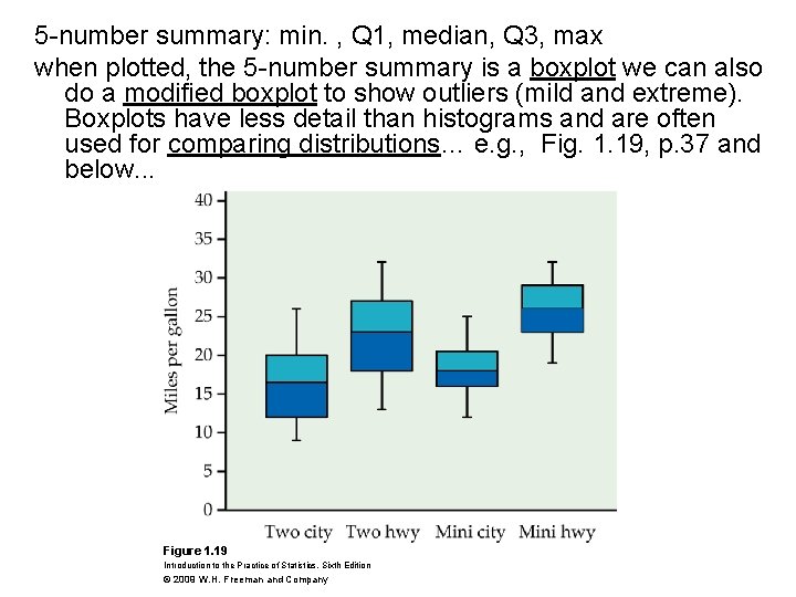
5 -number summary: min. , Q 1, median, Q 3, max when plotted, the 5 -number summary is a boxplot we can also do a modified boxplot to show outliers (mild and extreme). Boxplots have less detail than histograms and are often used for comparing distributions… e. g. , Fig. 1. 19, p. 37 and below. . . Figure 1. 19 Introduction to the Practice of Statistics, Sixth Edition © 2009 W. H. Freeman and Company

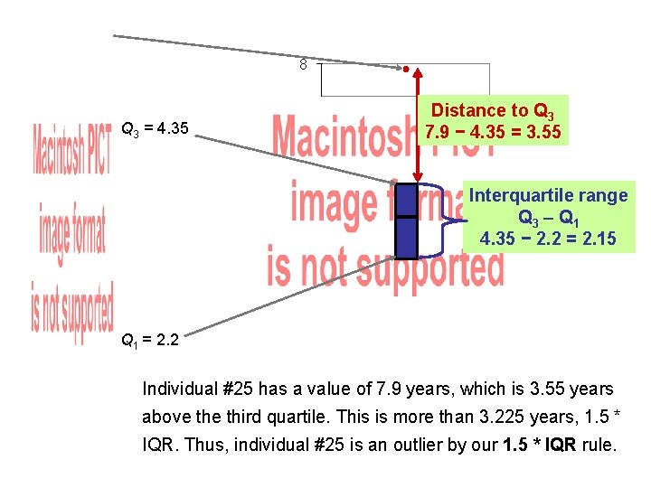
8 Q 3 = 4. 35 Distance to Q 3 7. 9 − 4. 35 = 3. 55 Interquartile range Q 3 – Q 1 4. 35 − 2. 2 = 2. 15 Q 1 = 2. 2 Individual #25 has a value of 7. 9 years, which is 3. 55 years above third quartile. This is more than 3. 225 years, 1. 5 * IQR. Thus, individual #25 is an outlier by our 1. 5 * IQR rule.

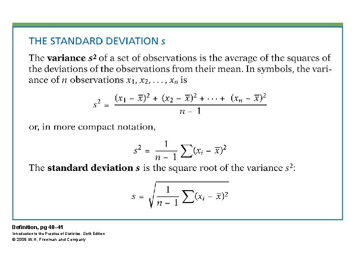
Definition, pg 40– 41 Introduction to the Practice of Statistics, Sixth Edition © 2009 W. H. Freeman and Company

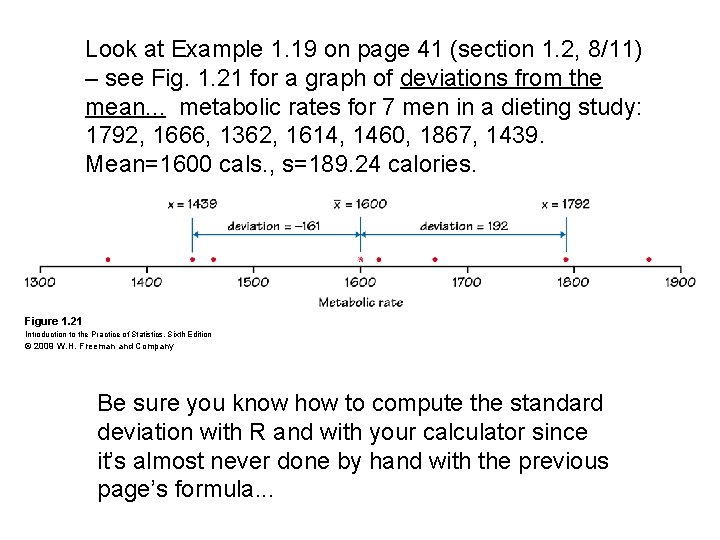
Look at Example 1. 19 on page 41 (section 1. 2, 8/11) – see Fig. 1. 21 for a graph of deviations from the mean. . . metabolic rates for 7 men in a dieting study: 1792, 1666, 1362, 1614, 1460, 1867, 1439. Mean=1600 cals. , s=189. 24 calories. Figure 1. 21 Introduction to the Practice of Statistics, Sixth Edition © 2009 W. H. Freeman and Company Be sure you know how to compute the standard deviation with R and with your calculator since it’s almost never done by hand with the previous page’s formula. . .

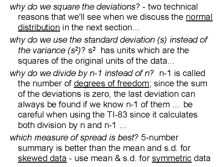
why do we square the deviations? - two technical reasons that we'll see when we discuss the normal distribution in the next section… why do we use the standard deviation (s) instead of the variance (s 2)? s 2 has units which are the squares of the original units of the data… why do we divide by n-1 instead of n? n-1 is called the number of degrees of freedom; since the sum of the deviations is zero, the last deviation can always be found if we know n-1 of them … be careful when using the TI-83 since it calculates both division by n and n-1 … which measure of spread is best? 5 -number summary is better than the mean and s. d. for skewed data - use mean & s. d. for symmetric data

Some R commands that will be useful in doing these computations: mean(X); median(X); sd(X) ; min(X); max(X) sd(X)^2 #variance var(X) #also variance quantile(X) #gives quantiles for 0 -1 in steps of. 25 #to get others use probs= option - example below quantile(X, probs=c(0, . 025, . 05, . 25, . 75, . 975, 1)) IQR(X) #gives the interquartile range of X # #use scan() to read in a small number of a single #variable. Hit "Enter" twice to end the data entry… scan() # use the square brackets to subset a dataframe

What should you use, when, and why? Arithmetic mean or median? • Middletown is considering imposing an income tax on citizens. City hall wants a numerical summary of its citizens income to estimate the total tax base. – Mean: Although income is likely to be right-skewed, the city government wants to know about the total tax base. • In a study of standard of living of typical families in Middletown, a sociologist makes a numerical summary of family income in that city. – Median: The sociologist is interested in a “typical” family and wants to lessen the impact of extreme incomes.

• Finish reading section 1. 2 • Be sure to go over the Summary at the end of each section and know all the terminology • Do # 1. 56, 1. 62 -1. 64, 1. 67, 1. 69, 1. 75 -1. 77 (Mean/Median Applet), 1. 78, 1. 79 • use R for any problem requiring more than very simple computations… or use the TI 83 for numerical (but not graphical) analysis. . .