Numerical black hole simulations Luis Lehner LSU NSFNASASloanResearch
![Numerical ‘black hole’ simulations Luis Lehner LSU [NSF-NASA-Sloan-Research Corporation]](https://slidetodoc.com/presentation_image_h2/b850460de4b003331f01a6c1f6c94415/image-1.jpg "Numerical ‘black hole’ simulations Luis Lehner LSU [NSF-NASA-Sloan-Research Corporation]")
Numerical ‘black hole’ simulations Luis Lehner LSU [NSF-NASA-Sloan-Research Corporation]

Overview • Status of ‘basic’ efforts – What we know & would like to know at continuum level – From continuum to discrete – Head-ways/messages to other disciplines • Status through 3 examples (3, 2, 1 + time dimensions). From ‘qualitative’ to precision physics…. – Astrophysical black hole simulations – Higher dimensional black holes and related systems • Final comments

Where are we now ‘The good, the bad and the ugly’ • Initial value problem: Advanced on development, analysis and use of formulations of Einstein equations. – Previously used equations were weakly hyperbolic generically ill-posed! – Can be ‘fixed’ by adding constraints (and coord conditions) in a suitable manner – Yet, lots of possibilities, ‘infinitely’ many different formulations. • Poor’s man way: parameter search, dynamical adjusting them, and/or ‘cleanup’ constraints. Tiglio, LL, Neilsen
![• Initial value boundary problem: Well posedness established [Friedrich-Nagy]. – Allows for specifying](http://slidetodoc.com/presentation_image_h2/b850460de4b003331f01a6c1f6c94415/image-4.jpg "• Initial value boundary problem: Well posedness established [Friedrich-Nagy]. – Allows for specifying")
• Initial value boundary problem: Well posedness established [Friedrich-Nagy]. – Allows for specifying the ‘right’ boundary –physical– data. Just one formulation where this is known at the non-linear level – A couple of others at linear level, well posed but unable to specify desired boundary condition • Poor’s man way of dealing with this: Push boundaries far out. • A more refined way, understand well posedness of underlying problem with suitable boundary conditions. For radiative ones, in a standard formulation elliptic gauge equation to rule out weak (polynomial) instability [Sarbach-Reula in a model problem]. • For global problem. Reach future null infinity by matching formulations or conformal eqns.

Moving to numerical arena • Guiding principle: reproduce analytical steps at ‘all’ cost. – System: – What’s involved here? – Why did we get this? – Numerically? Obtain a (semi-) discrete energy estimate • • • Operator? Boundaries? Dissipation? • Integration in time. RK 3 -RK 4 preserves the discrete energy stability! Gustaffson-Kreiss-Oliger; Strand; Olsson; Tadmor Calabrese-L. L. -Neilsen-Pullin-Reula-Sarbach-Tiglio

Example 1 • Binary black hole simulations. – Leading edge, a few efforts leading to ‘orbits’. • Rationale, use what is available the ‘best’ possible way and push ahead the problem at hand. – F. Pretorius effort: • Einstein eqns in harmonic coordinates. • Adaptive mesh refinement to achieve high resolution near black holes • Addition of constraint terms to ‘damp’ spurious growth. [H. Friedrich, Sarbach-Tom]

• Generalized harmonic coordinates introduce a set of arbitrary source functions H u into the usual definition of harmonic coordinates • With H u regarded as independent functions, the principle part of the equation for each metric element reduces to a simple wave equation • Constraints: • Behavior? • To help with constraint’s growth, modify eqns by adding constraints [Gundach et al, following Brodbeck-Huebner-Reula-Frittelli]

Effect of damping terms • Axisymmetric simulation of a Schwarzschild black hole, Painleve-Gullstrand coords. • Left and right simulations use identical parameters except for the use of constraint damping • Not ‘robust’ for al problems

status, prospects…. • ‘Realistic’ initial data still unknown, presently trying to understand generic features of binary black hole mergers – Initial data defined by boosted over-critical scalar field configurations. – choice for initial geometry and scalar field profile: • spatial metric and its first time derivative is conformally flat • maximal (gives initial value of lapse and time derivative of conformal factor) and harmonic (gives initial time derivatives of lapse and shift) • Hamiltonian and Momentum constraints solved for initial values of the conformal factor and shift, respectively – advantages of this approach • “simple” in that initial time slice is singularity free • all non-trivial initial geometry is driven by the scalar field—when the scalar field amplitude is zero he recovers Minkowski spacetime – disadvantages • ad-hoc in choice of parameters to produce a desired binary system • uncontrollable amount of “junk” initial radiation (scalar and gravitational) in the spacetime; though all present initial data schemes suffer from this to some degree. – Numerical ingredients • Adaptive mesh refinement technique employed • ‘Compactification’ of spatial coordinates + artificial dissipation to wipe out everything that leaves sufficiently far.

‘dynamics’ • Initially: – – – – • equal mass components eccentricity e ~ 0 - 0. 2 coordinate separation of black holes ~ 13 M proper distance between horizons ~ 16 M velocity of each black hole ~0. 16 spin angular momentum = 0 ADM Mass ~ 2. 4 M Final black hole: – Mf ~ 1. 9 M – Kerr parameter a ~ 0. 70 – ‘error’ ~ 5%
 coordinates")
Scalar field f. r, uncompactified coordinates Scalar field f. r, compactified (code) coordinates
 coordinates Reduced mass frame; heavier lines are position of BH")
Simulation (center of mass) coordinates Reduced mass frame; heavier lines are position of BH 1 relative to BH 2 (green star); thinner black lines are reference ellipses

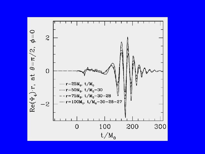
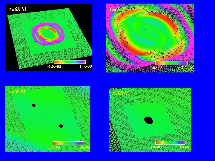
Real component of the Newman-Penrose scalar Y 4 times r, x=0 slice of the solution Real component of the Newman-Penrose scalar Y 4 times r, z=0 slice of the solution

Summary of computation – medium resolution simulation • base grid resolution 333 – 9 levels of 2: 1 mesh refinement (effective finest grid resolution of 81923) … switched to 8 levels maximum at around 150 M – ~ 50, 000 time steps on finest level – ~550 hours on 48 nodes of UBC’s vnp 4 Xeon cluster (26, 000 CPU hours total) – maximum total memory usage ~ 10 GB, disk usage ~ 100 GB (and this is very infrequent output!)

Pushing ahead… Zoom-whirl ? finite number of ‘humps’

Notes…. • ‘First-sight’ prognosis… bbh orbits underway. Some qualitative, semiquantitative answers coming and in the way. • Estimates of expected growth can play a major role: – to discern among different formulations – to exploit this knowledge at the numerical level • How must one deal with ‘non-constant’ characteristic structure? – e. g. u, t=f(x, y) u, x with f(x=0, y) = sin(y) • Existing/gained knowledge spilling out to close fields – Eg. MHD eqns often used are weakly hyperbolic, upon re-expression yield vastly improved simulations without ‘special tricks’ [Hirschman-Neilsen-Reula-LL] • Every simulation still require large resources – too long times–. Further developments in numerics/computational techniques to come.

‘lower’ the dimensionality by going higher…

Black strings and bubbles • Black strings: higher dimensional black holes. In 5 D black holes with ‘maximum’ symmetries are : S 3 hyperspherical black hole or S 2 x. R cylindrical black hole or black string. • Bubbles. Topogically ‘weird’ spacetimes. – An initially large sphere can’t be shrank to zero size – Minkowski spacetime shown to be able to ‘quantum tunnel’ to a bubble spacetime (Witten bubble) • Studying both systems require numerical simulations of Einstein equations in higher dimensions (5 D) but symmetries allow for treating the black string in 2+1 and bubble in 1+1 dimensions.

Black strings 1. - Contain singularities 2. - Ruled by null-rays 3. - Non-unique even in spherical symm Stability? - Black string perturbations admit exponential growth for L > Lc (Gregory-Laflamme) - Entropy SBS<SBH (for a given M) Conjecture: Black strings will bifurcate

• Conjecture used in many scenarios • Density of states from Ads/CFT correspondence • Discussions of BH on brane worlds. BH in matrix theory, etc Recent developments • Horowitz-Maeda, can’t bifurcate in finite time. Conjecture: will ‘settle’ to a non-uniform stationary soln (ie. No bifurcation in infinite affine time) • Gubser: transition to soln of first-order type in 5 -6 D (1 st, ~2 nd order pert) • Wiseman: stationary solns which are not the Horowitz-Maeda ones. • Kol: Transition from black string to BH through a conical singularity • Sorkin-Kol: for high enough dimensions transition is of 2 nd order. • Qns: – What is the final solution of a perturbed black string? – Can it bifurcate in ‘infinite time’? – Are Wiseman’s solns, physically relevant?

Some details • • Spherical symmetry 2+1 problem. BUT a priori quite a zoo of possibilities! Line element: • Initial data – • Solve constraints with a seed perturbation in gqq Boundary? – Might need to ‘evolve’ for very long!. ‘Compactify’ r direction (dissipation needed)

Monitoring the evolution • Apparent horizon & Null surfaces • Kretschmann invariant I=Rabcd – For BS, at ev. horizon: IA = 12/R 4 ; – For hyperspherical BH at ev horizon: IA = 72/R 4 – Monitor I R 4/12 {1, 6} for {BS, hyper. BH} • Excision at: – RAH – buffer – min(RAH) – buffer Checked evolution independence on choice made • Radial resolution near app horizon ~ M/(200 x n) {n=1. . 8} [Choptuik, LL, Olabarrieta, Pretorius, Petryk, Villegas]

Super-critical case

Curvature ‘Event’ horizon
 • “bifurcation” in infinite affine time")
• Affine time, l=es growing exponentially (~1022) • “bifurcation” in infinite affine time certainly possible • ‘cascade’ of unstable strings also possible [Garfinkle-LL-Pretorius]
 requires existence of certain (asymptotically")
• Problem: Kaluza-Klein ‘bubbles’ –Positive mass thm (Witten) requires existence of certain (asymptotically constant) spinors. In 5 d Kaluza-Klein theory (asymptotically R 3 x. S 1) these spinors are not guaranteed. 1. Are there negative mass configurations? 2. Is cosmic censorship valid? • Answer to 1. Yes, negative mass configurations found –Witten bubble (82): associated with instability of KK vacuum. More than 1 state with zero total energy. –Brill-Pfister (89): explicit solutions to 5 D vacuum constraints with negative mass. –Brill-Horowitz (91): generalization to include ‘gauge’ fields. • Qn: What’s the space-time like? –Corley-Jacobson (94). Analyze area of the bubble, conclusion: It starts out expanding [collapsing], if this trend continues, unlikely to form a singularity. • Conjecture: It will keep expanding [collapsing] out (otherwise go through another moment of time symmetry). • But…. . This only from estimates at the initial hypersurface… what does really happen? … Need to solve the eqns… –Numerical effort (2000). Conclusion: negative mass bubbles expand but not forever…. At some point a naked singularity appears!!! (or does it? )
 0 (for r=r+ ) a smooth function")
Revisiting the problem • Consider: With U(r) 0 (for r=r+ ) a smooth function (U 1 asymptotically) Bubble is at r+. Electrovac case, consider Time symmetry (mom const =0); Hamiltonian constraint With m, b constants. In particular MADM=m/4…but this can be negative Initial acceleration of the bubble’s area [extending Corley-Jacobson] • • n=2. If m<0, bubble expands; m>0 both cases possible n>2. For k large, arbitrary negative acceleration with negative mass…sounds promising! Sarbach, LL PRD 03; 05.
 only (1 D evolution) • Understood")
Numerical evolution • Variables functions of (t, r) only (1 D evolution) • Understood constraint growth and suitable boundary conditions [a-la Calabrese, LL, Tiglio 02] • At bubble, regularity conditions used. • Proved well posedness at continuum level, translated to the numerical arena thanks to SBP in a first order formulation. • Improved resolution at bubble with a non-uniform radial coordinate. k=0 Case studied numerically previously, no naked singularity found, m<0 expands even faster than m>0

More than we asked for… What happens with a non-zero gauge field? • Choose n=2, and stick to cases where bubble starts out collapsing (positive mass) Depending on field strength, the bubble either collapses (k<k*) to a black string or bounces back to expand (k>k*). Changes behavior almost always without going through another moment of time symmetry Last… it appears to approach a stationary solution… does it exist?

Curvature invariant, sub/supra critical behavior Observation… there must be a static solution at the threshold
; U=(1 -r+/r).")
• Put static anzats, solve resulting constraint and… With V=(1 -r-/r); U=(1 -r+/r). And the parameters are obtained from P=4 pr+(1 -r-/r+)(3/2) and M=r+/4. • New solution? … nah… obtained by ‘just’ analytically continuing that of a charged black string…. [found in Horowitz-Maeda 03] • Analyzed spectrum of operator and confirmed a single growing mode f ~ ekt • Pulsation operator, upper/lower bounds within a suitable Hilbert space, Sturm-Liouville type problem • Upon : t iz, z it f ~ eikz, k ~ 1/Lc • Used to show a family of charged black strings becomes more unstable as charged is added (opposite to what was conjectured)

• What happened with the negative mass data that started contracting with arbitrary negative acceleration? – Bubble shrinks to arbitrarily small sizes, but ‘bounces’ back… cosmic censorship stood its ground

Final words • Numerical relativity can indeed provide ‘experimental’ set-up and pose new questions • Critical phenomena • Cosmology • Bubble/black string problem • Robust ‘generic’ implementations of Einstein equations will benefit (a lot!) from extra input ‘analytically’ obtained • Estimates including lower order terms (problem dependent, but technique? ) • Estimates including constraint growth (or how to control them) • Constraint preserving boundary conditions or how to go around them • Radiative boundary conditions (no theory so far), how to proceed with nonconstant characteristics? • Translation of the above to numerics, implementation, resolution, etc + all the ‘extracan-of-worms’ that come with this. • In the mean time, we’ll do the best we can!
- Slides: 36