Numerical Analysis Lecture 40 Chapter 7 Ordinary Differential

Numerical Analysis Lecture 40

Chapter 7 Ordinary Differential Equations

Introduction Taylor Series Euler Method Runge-Kutta Method Predictor Corrector Method

RUNGAKUTTA METHODS

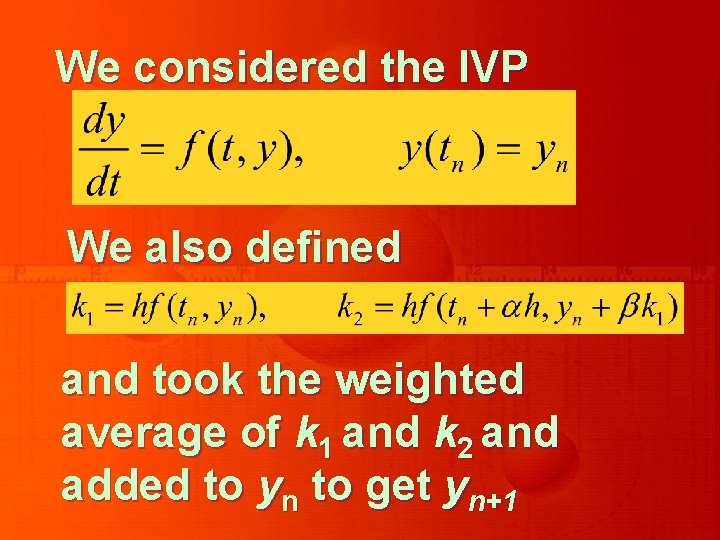
We considered the IVP We also defined and took the weighted average of k 1 and k 2 and added to yn to get yn+1

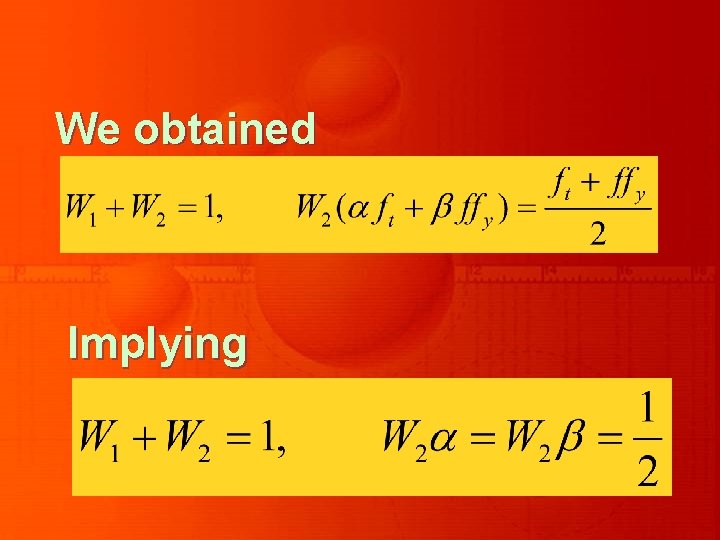
We obtained Implying

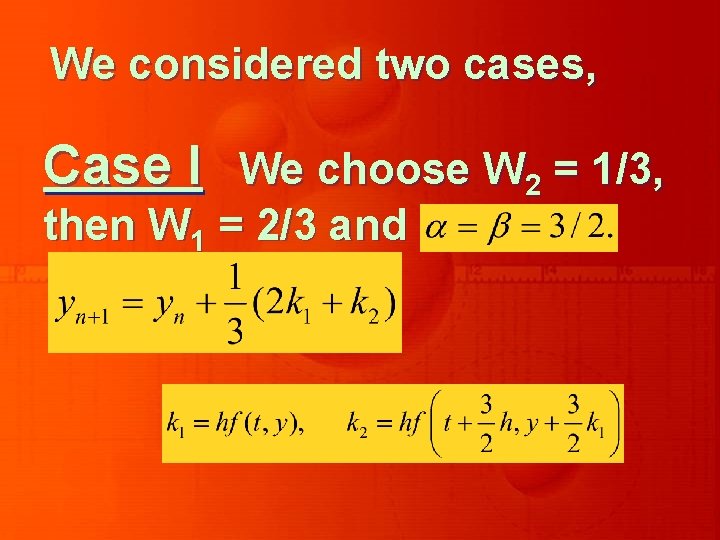
We considered two cases, Case I We choose W 2 = 1/3, then W 1 = 2/3 and

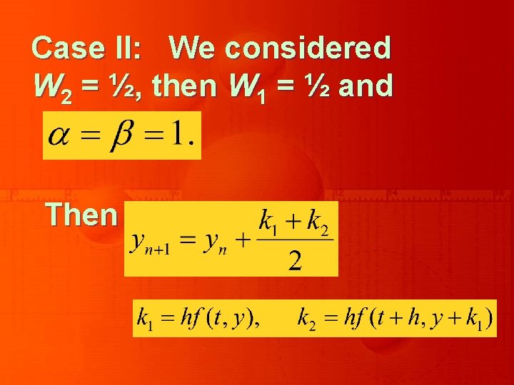
Case II: We considered W 2 = ½, then W 1 = ½ and Then

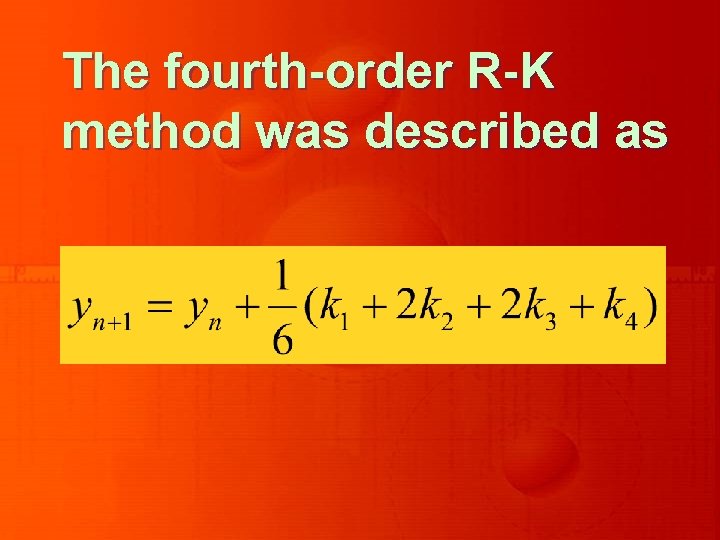
The fourth-order R-K method was described as

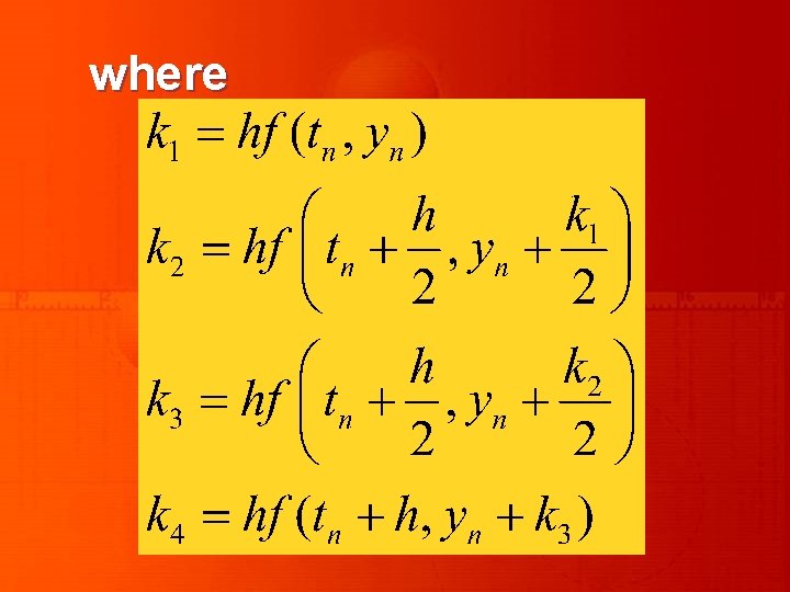
where

PREDICTOR – CORRECTOR METHOD

Milne’s Method It is a multi-step method where we assume that the solution to the given IVP is known at the past four equally spaced point t 0, t 1, t 2 and t 3.

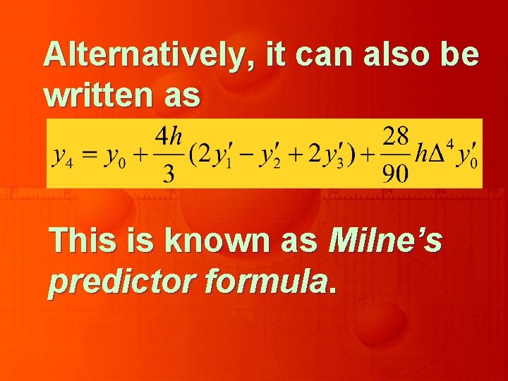
Alternatively, it can also be written as This is known as Milne’s predictor formula.

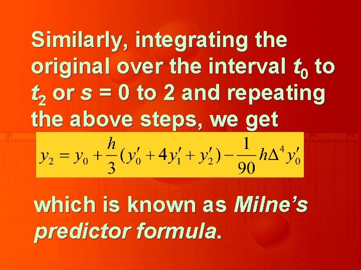
Similarly, integrating the original over the interval t 0 to t 2 or s = 0 to 2 and repeating the above steps, we get which is known as Milne’s predictor formula.

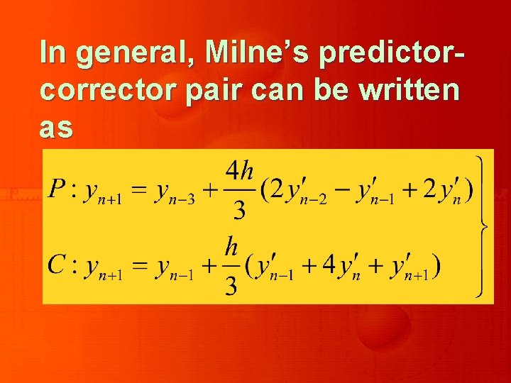
In general, Milne’s predictorcorrector pair can be written as

Adam-Moulton Method It is another predictorcorrector method, where we use the fact that the solution to the given initial value problem is known at past four equally spaced points tn, tn-1, tn-2, tn-3.

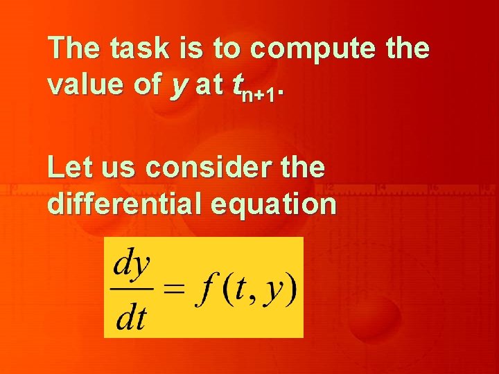
The task is to compute the value of y at tn+1. Let us consider the differential equation

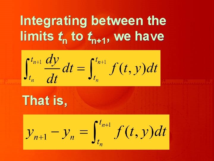
Integrating between the limits tn to tn+1, we have That is,

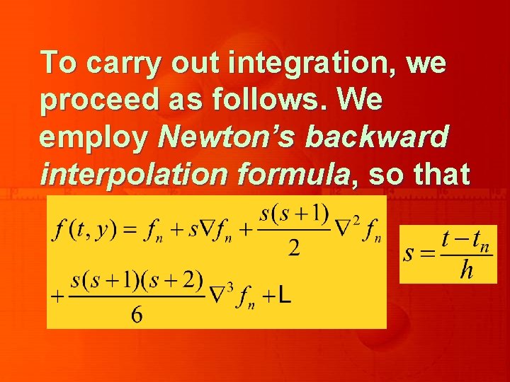
To carry out integration, we proceed as follows. We employ Newton’s backward interpolation formula, so that

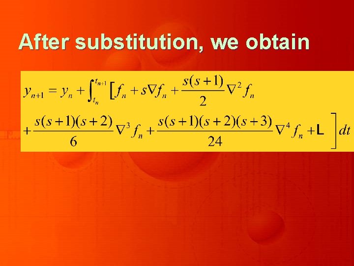
After substitution, we obtain

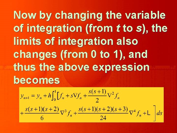
Now by changing the variable of integration (from t to s), the limits of integration also changes (from 0 to 1), and thus the above expression becomes

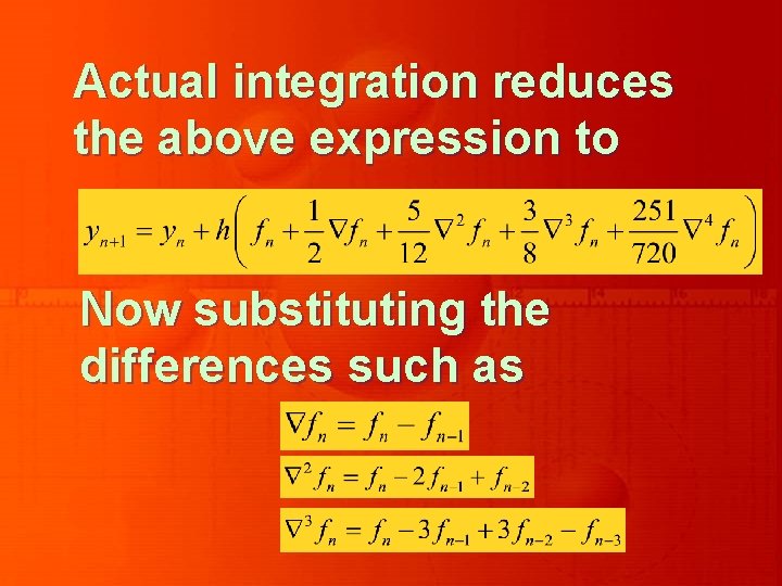
Actual integration reduces the above expression to Now substituting the differences such as

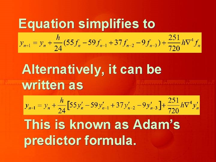
Equation simplifies to Alternatively, it can be written as This is known as Adam’s predictor formula.

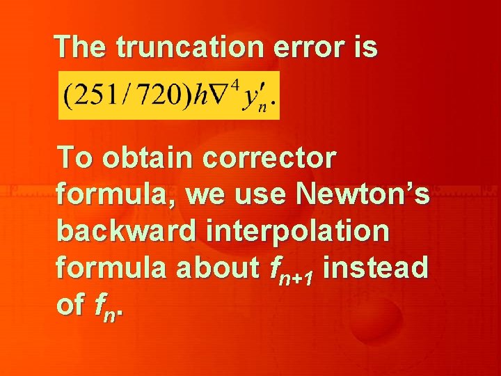
The truncation error is To obtain corrector formula, we use Newton’s backward interpolation formula about fn+1 instead of fn.

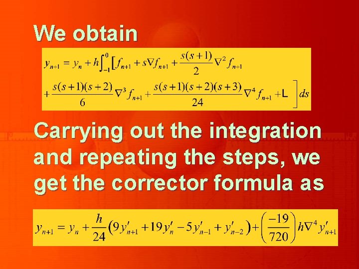
We obtain Carrying out the integration and repeating the steps, we get the corrector formula as

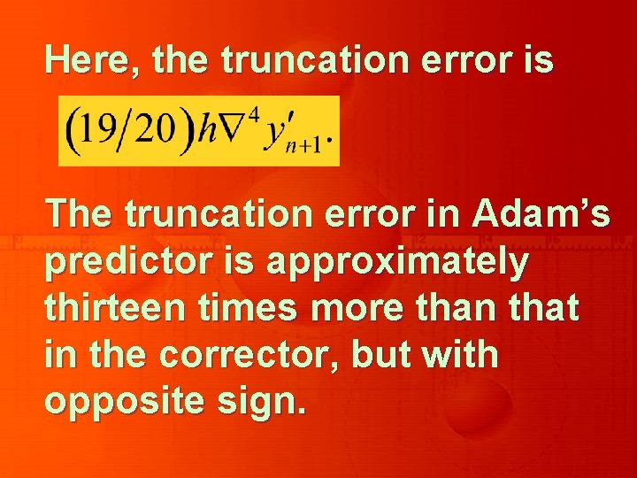
Here, the truncation error is The truncation error in Adam’s predictor is approximately thirteen times more than that in the corrector, but with opposite sign.

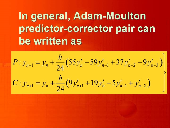
In general, Adam-Moulton predictor-corrector pair can be written as

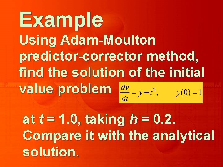
Example Using Adam-Moulton predictor-corrector method, find the solution of the initial value problem at t = 1. 0, taking h = 0. 2. Compare it with the analytical solution.

Solution In order to use Adam’s P-C method, we require the solution of the given differential equation at the past four equally spaced points, for which we use R-K method of 4 th order which is self starting.

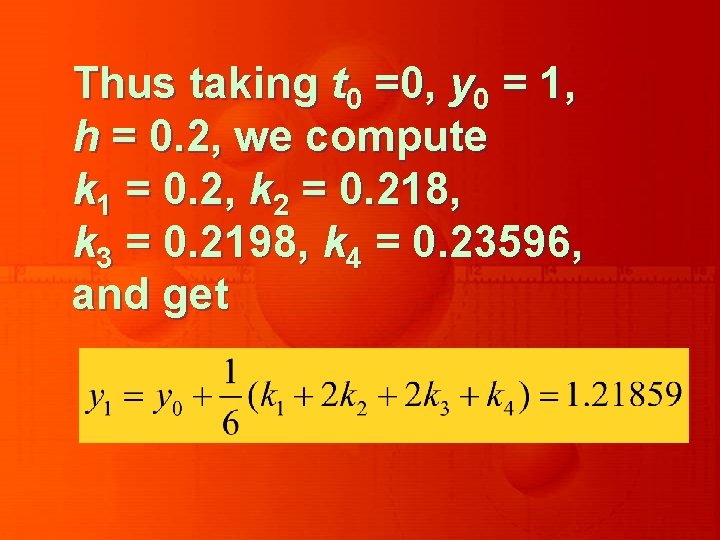
Thus taking t 0 =0, y 0 = 1, h = 0. 2, we compute k 1 = 0. 2, k 2 = 0. 218, k 3 = 0. 2198, k 4 = 0. 23596, and get

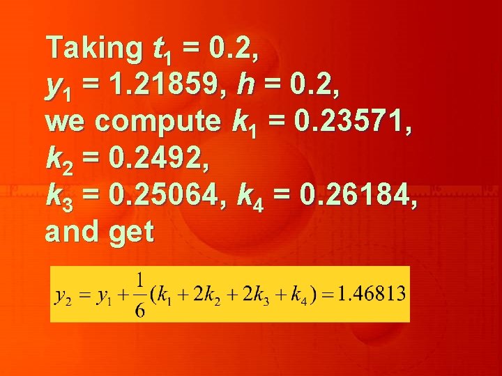
Taking t 1 = 0. 2, y 1 = 1. 21859, h = 0. 2, we compute k 1 = 0. 23571, k 2 = 0. 2492, k 3 = 0. 25064, k 4 = 0. 26184, and get

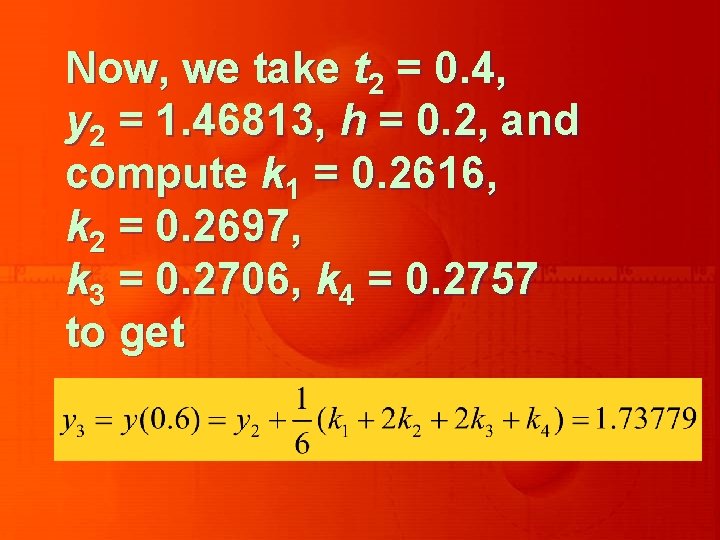
Now, we take t 2 = 0. 4, y 2 = 1. 46813, h = 0. 2, and compute k 1 = 0. 2616, k 2 = 0. 2697, k 3 = 0. 2706, k 4 = 0. 2757 to get

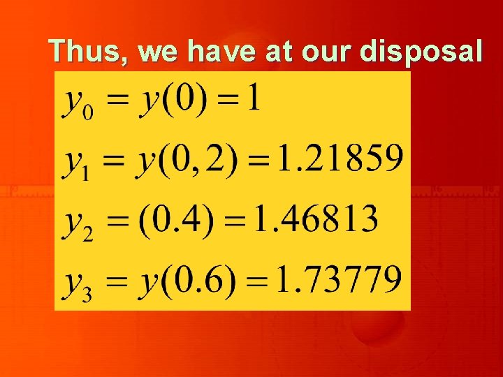
Thus, we have at our disposal

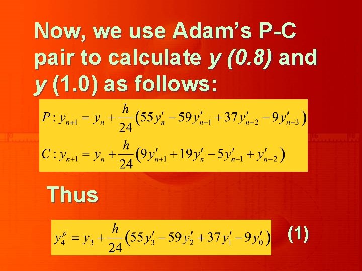
Now, we use Adam’s P-C pair to calculate y (0. 8) and y (1. 0) as follows: Thus (1)

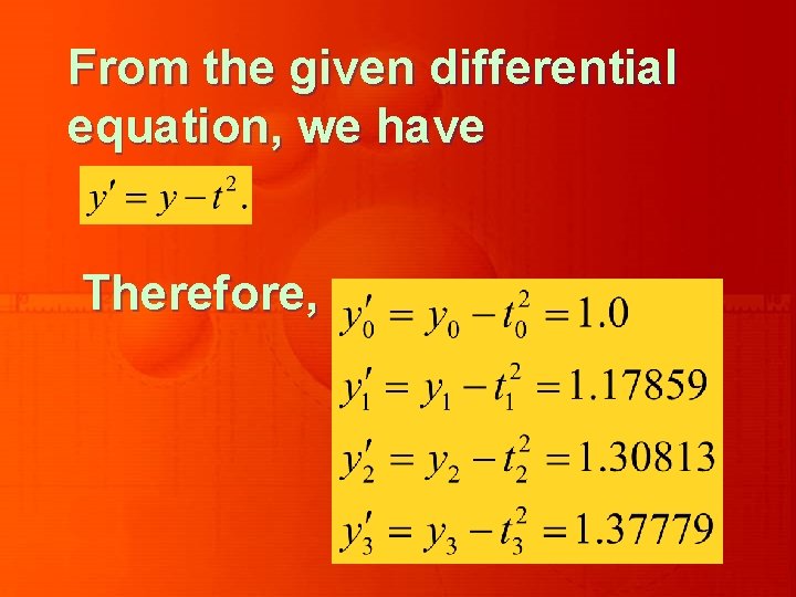
From the given differential equation, we have Therefore,

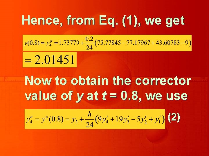
Hence, from Eq. (1), we get Now to obtain the corrector value of y at t = 0. 8, we use (2)

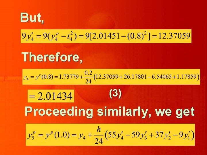
But, Therefore, (3) Proceeding similarly, we get

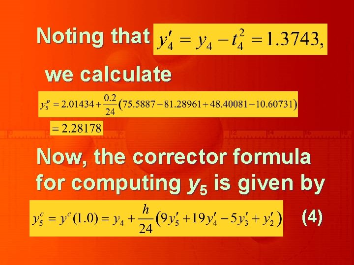
Noting that we calculate Now, the corrector formula for computing y 5 is given by (4)

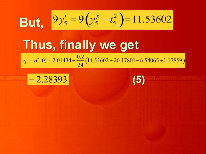
But, Thus, finally we get (5)

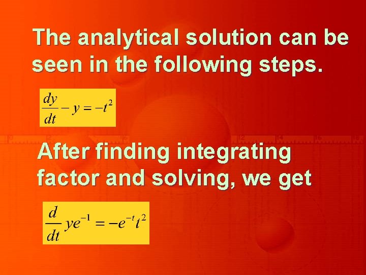
The analytical solution can be seen in the following steps. After finding integrating factor and solving, we get

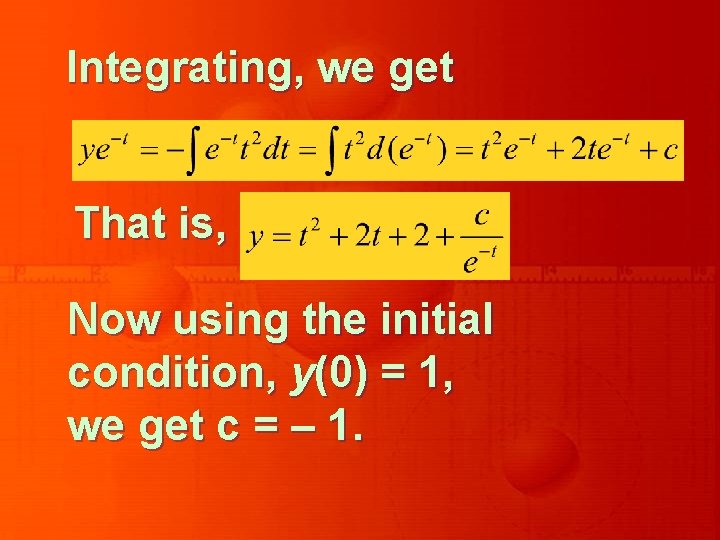
Integrating, we get That is, Now using the initial condition, y(0) = 1, we get c = – 1.

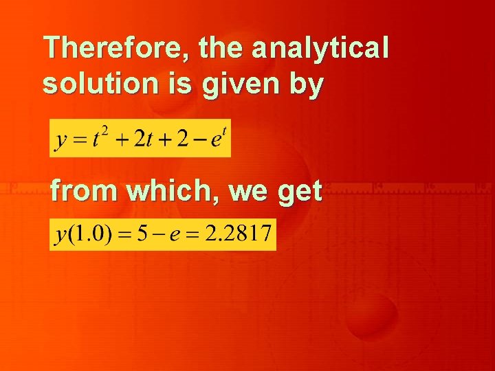
Therefore, the analytical solution is given by from which, we get

Convergence and Stability Considerations

The numerical solution of a differential equation can be shown to converge to its exact solution, if the step size h is very small.

The numerical solution of a differential equation is said to be stable if the error do not grow exponentially as we compute from one step to another.

Stability consideration are very important in finding the numerical solutions of the differential equations either by single-step methods or by using multistep methods.

However, theoretical analysis of stability and convergence of R -K methods and P –C methods are highly involved and obtain numerically stable th solution using 4 order R – K method to the simple problem y’ = Ay gives us stability condition as -2. 78<Ah

In practice, to get numerically stable solutions to similar problems, we choose the value of h much smaller than the value given by the above condition and also check for consistency of the result.

Another topic of interest which is not considered, namely the stiff system of differential equations that arises in many chemical engineering systems, such as chemical reactors, where the rate constants for the reactions involved are widely different.

Most of the realistic stiff DE do not have analytical solutions and therefore only numerical solutions can be obtained.

However, to get numerically stable solutions, a very small step size h is required, to use either R-K methods or P – C methods. More computer time is required

Numerical Analysis Lecture 40