Numerical Analysis Lecture 25 Chapter 5 Interpolation Finite





- Slides: 53

Numerical Analysis Lecture 25

Chapter 5 Interpolation

Finite Difference Operators Newton’s Forward Difference Interpolation Formula Newton’s Backward Difference Interpolation Formula Lagrange’s Interpolation Formula Divided Differences Interpolation in Two Dimensions Cubic Spline Interpolation

Newton’s Forward Difference Interpolation Formula


An alternate expression is

NEWTON’S BACKWARD DIFFERENCE INTERPOLATION FORMULA

The formula is,

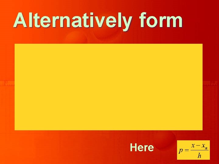
Alternatively form Here

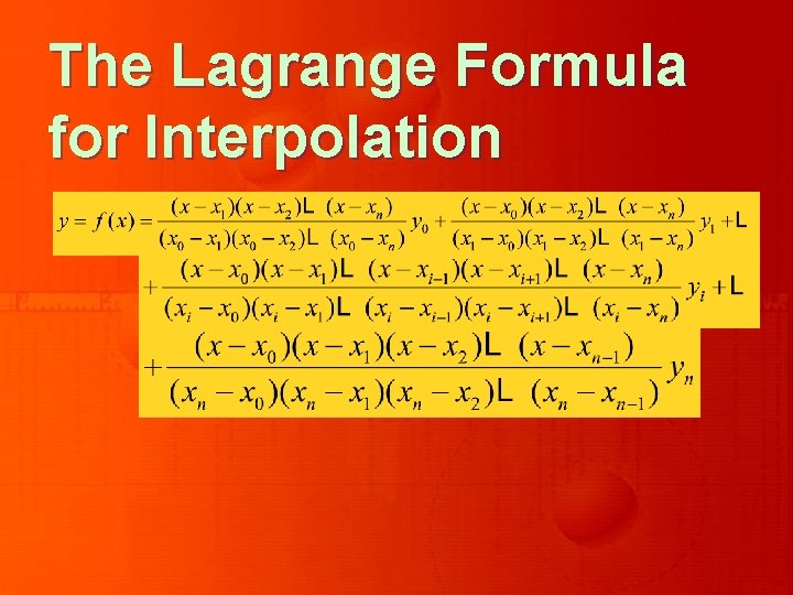
LAGRANGE’S INTERPOLATION FORMULA

The Lagrange Formula for Interpolation

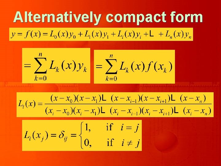
Alternatively compact form

Also

Finally, the Lagrange’s interpolation polynomial of degree n can be written as

DIVIDED DIFFERENCES

Let us assume that the function y = f (x) is known for several values of x, (xi, yi), for i=0, 1, . . n. The divided differences of orders 0, 1, 2, …, n are now defined recursively as:

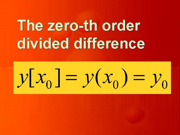
The zero-th order divided difference

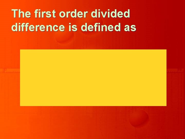
The first order divided difference is defined as

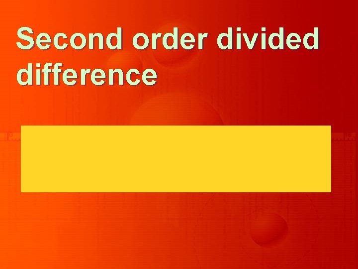
Second order divided difference

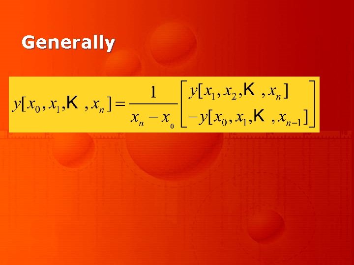
Generally

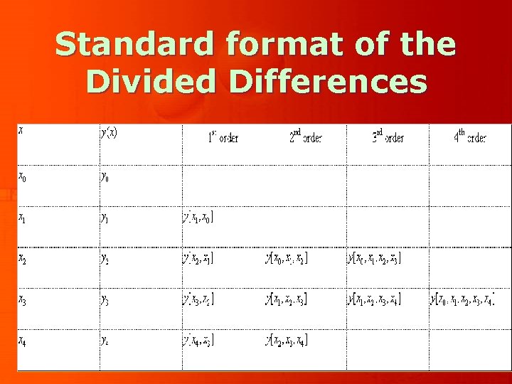
Standard format of the Divided Differences

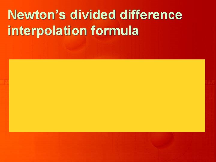
NEWTON’S DIVIDED DIFFERENCE INTERPOLATION FORMULA

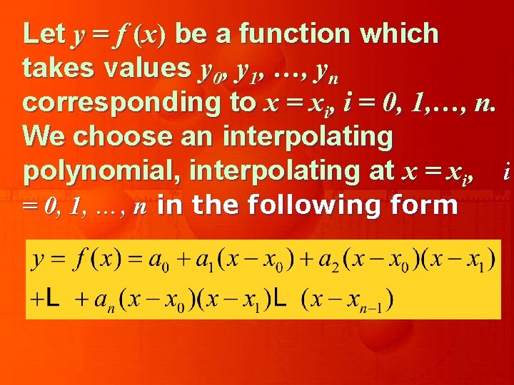
Let y = f (x) be a function which takes values y 0, y 1, …, yn corresponding to x = xi, i = 0, 1, …, n. We choose an interpolating polynomial, interpolating at x = xi, i = 0, 1, …, n in the following form

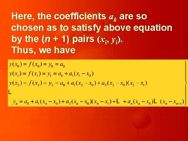
Here, the coefficients ak are so chosen as to satisfy above equation by the (n + 1) pairs (xi, yi). Thus, we have

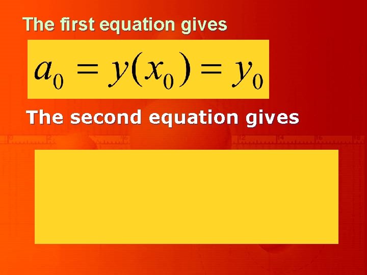
The first equation gives The second equation gives

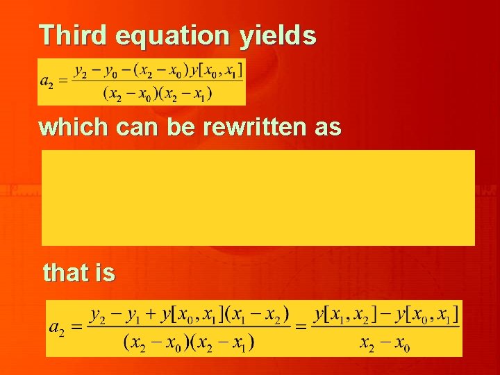
Third equation yields which can be rewritten as that is

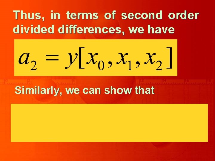
Thus, in terms of second order divided differences, we have Similarly, we can show that

Newton’s divided difference interpolation formula

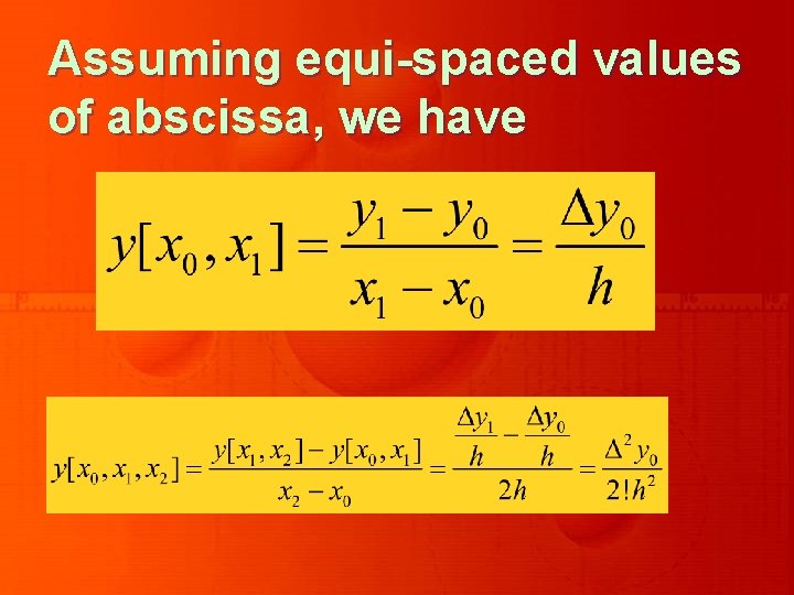
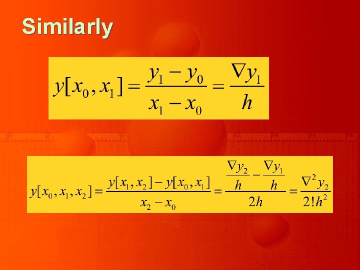
Newton’s divided differences can also be expressed in terms of forward, backward and central differences.

Assuming equi-spaced values of abscissa, we have

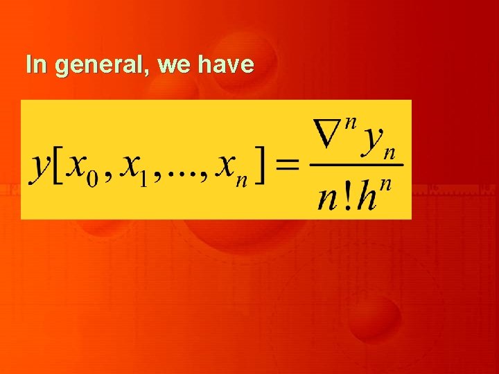
By induction, we can in general arrive at the result

Similarly

In general, we have

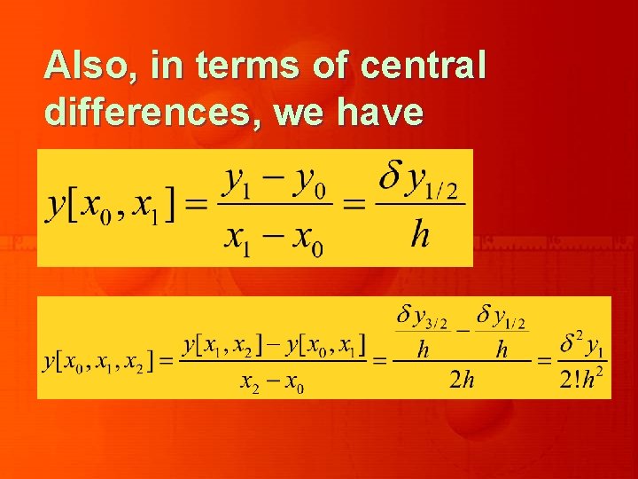
Also, in terms of central differences, we have

In general, we have the following pattern

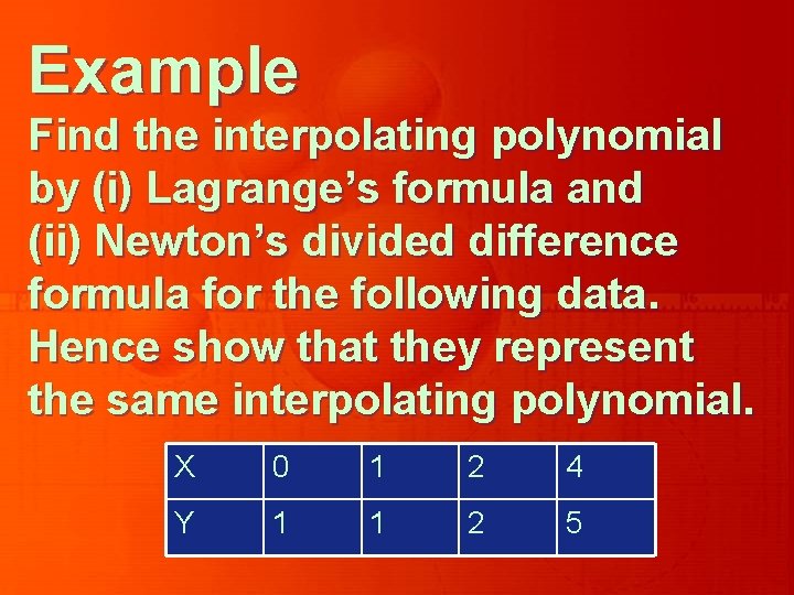
Example Find the interpolating polynomial by (i) Lagrange’s formula and (ii) Newton’s divided difference formula for the following data. Hence show that they represent the same interpolating polynomial. X 0 1 2 4 Y 1 1 2 5

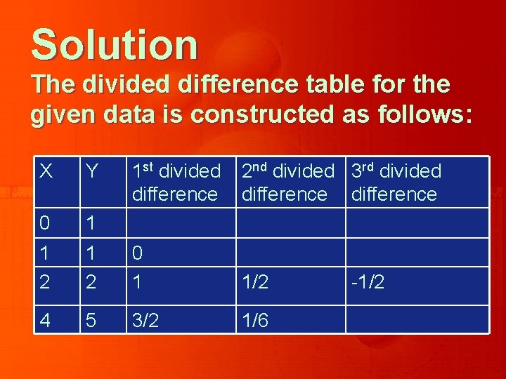
Solution The divided difference table for the given data is constructed as follows: X Y 1 st divided difference 2 nd divided 3 rd divided difference 0 1 1 2 0 1 1/2 4 5 3/2 1/6 -1/2

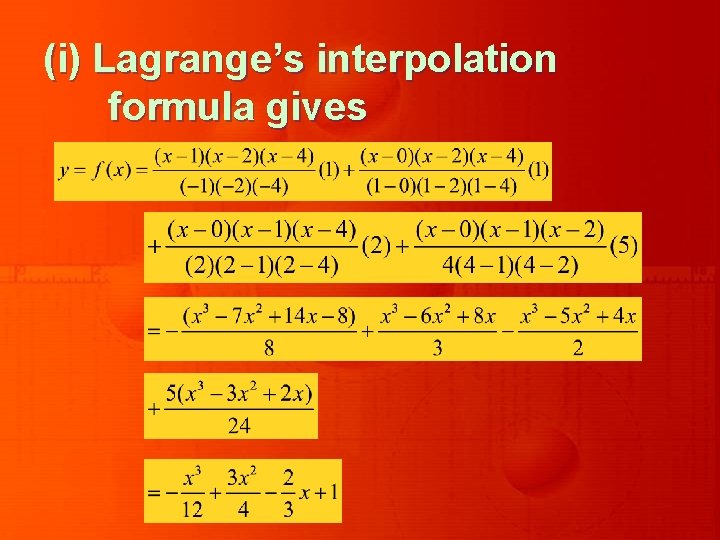
(i) Lagrange’s interpolation formula gives

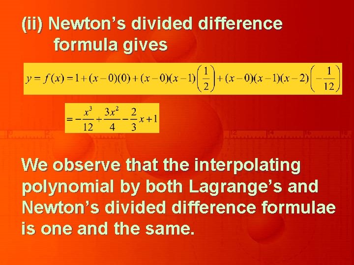
(ii) Newton’s divided difference formula gives We observe that the interpolating polynomial by both Lagrange’s and Newton’s divided difference formulae is one and the same.

Note! Newton’s formula involves less number of arithmetic operations than that of Lagrange’s.

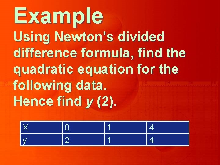
Example Using Newton’s divided difference formula, find the quadratic equation for the following data. Hence find y (2). X y 0 2 1 1 4 4

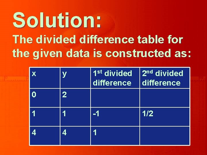
Solution: The divided difference table for the given data is constructed as: x y 1 st divided difference 2 nd divided difference 0 2 1 1 -1 1/2 4 4 1

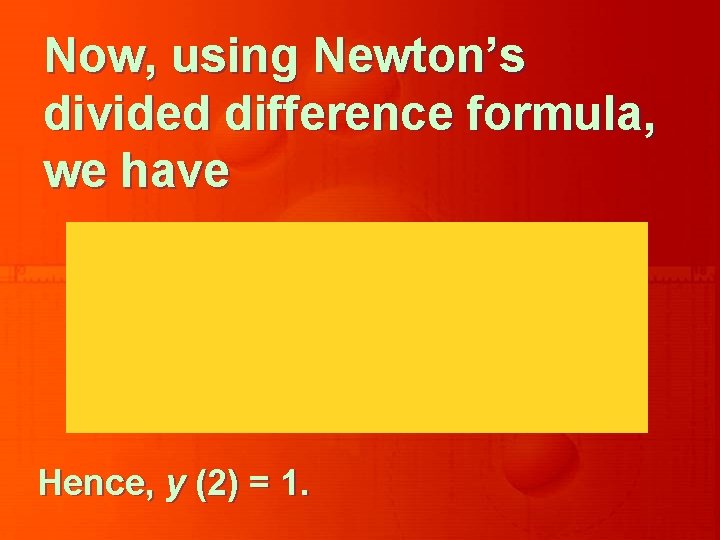
Now, using Newton’s divided difference formula, we have Hence, y (2) = 1.

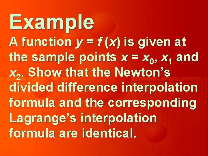
Example A function y = f (x) is given at the sample points x = x 0, x 1 and x 2. Show that the Newton’s divided difference interpolation formula and the corresponding Lagrange’s interpolation formula are identical.

Solution For the function y = f (x), we have the data

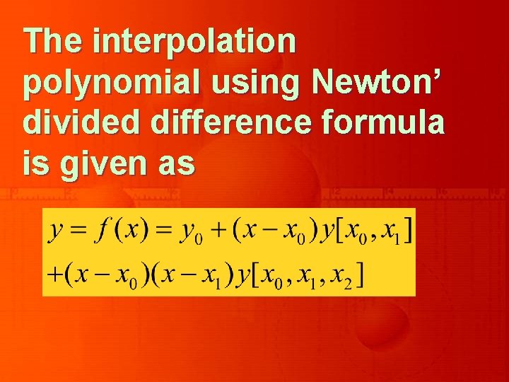
The interpolation polynomial using Newton’ divided difference formula is given as

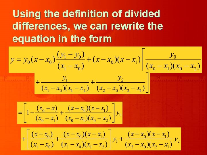
Using the definition of divided differences, we can rewrite the equation in the form

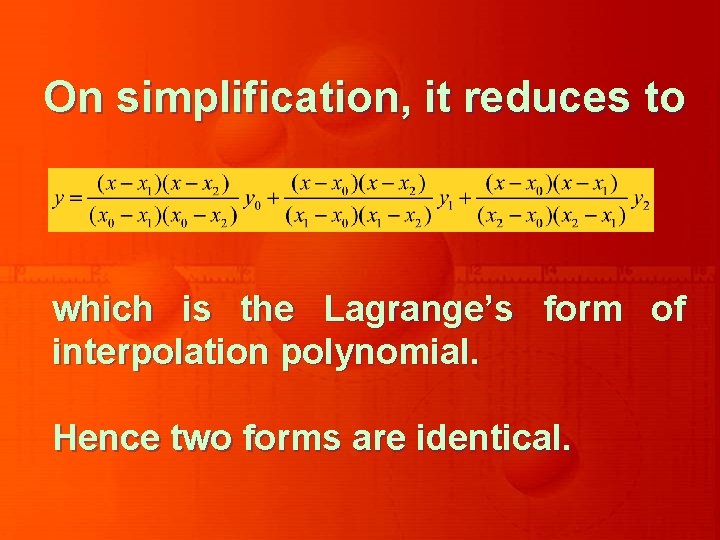
On simplification, it reduces to which is the Lagrange’s form of interpolation polynomial. Hence two forms are identical.

Newton’s Divided Difference Formula with Error Term

Following the basic definition of divided differences, we have for any x

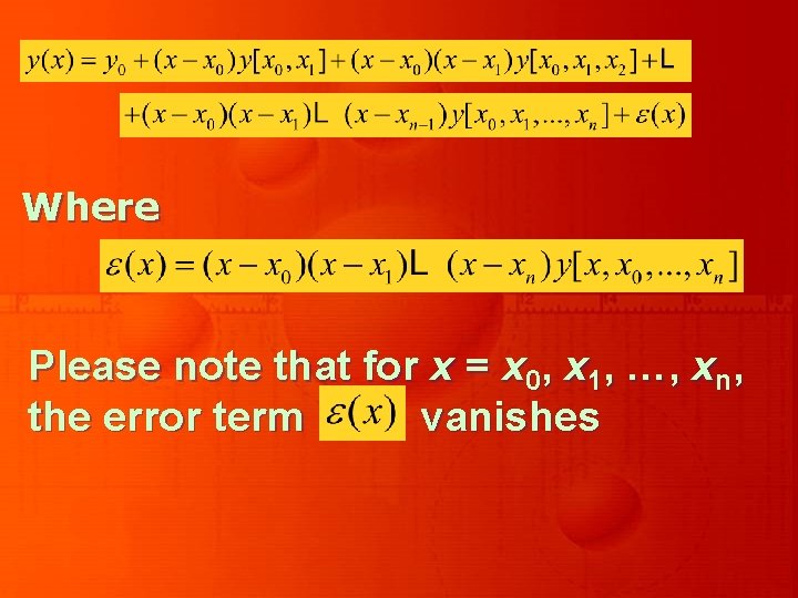
Multiplying the second Equation by (x – x 0), third by (x – x 0)(x – x 1) and so on, and the last by (x – x 0)(x – x 1) … (x – xn-1) and adding the resulting equations, we obtain

Where Please note that for x = x 0, x 1, …, xn, the error term vanishes

Numerical Analysis Lecture 25