Nuclear Magnetic Resonance NMR Probe the Composition Structure
 Probe the Composition, Structure, Dynamics and Function of the Complete")
Nuclear Magnetic Resonance (NMR) Probe the Composition, Structure, Dynamics and Function of the Complete Range of Chemical Entities: from small organic molecules to large molecular weight polymers and proteins. One of the MOST Techniques Routinely used Analytical
 elucidation • Natural product chemistry. • Synthetic organic")
Common NMR Utility • Structural (chemical) elucidation • Natural product chemistry. • Synthetic organic chemistry. Analytical tool of choice of synthetic chemists. • Study of dynamic processes • Reaction kinetics. • Study of equilibrium (chemical or structural). • Structural (three-dimensional) studies • Proteins. • DNA. Protein/DNA complexes • Polysaccharides • Drug design • Structure Activity Relationships by NMR • Medicine - MRI

NMR: “fingerprint” of the compound’s chemical structure 2 -phenyl-1, 3 -dioxep-5 -ene 1 H NMR spectra 13 C NMR spectra

Protein Structures from NMR 2 D NOESY Spectra at 900 MHz Lysozyme Ribbon Diagram

NMR History 1937 1946 1953 1966 1975 1985 Rabi predicts and observes nuclear magnetic resonance Bloch, Purcell first nuclear magnetic resonance of bulk sample Overhauser NOE (nuclear Overhauser effect) Ernst, Anderson Fourier transform NMR Jeener, Ernst 2 D NMR Wüthrich first solution structure of a small protein (BPTI) from NOE derived distance restraints 1987 3 D NMR + 13 C, 15 N isotope labeling of recombinant proteins (resolution) 1990 pulsed field gradients (artifact suppression) 1996/7 new long range structural parameters: - residual dipolar couplings from partial alignment in liquid crystalline media - projection angle restraints from cross-correlated relaxation TROSY (molecular weight > 100 k. Da) Nobel prizes 1944 Physics Rabi (Columbia) 1952 Physics Bloch (Stanford), Purcell (Harvard) 1991 Chemistry Ernst (ETH) 2002 Chemistry Wüthrich (ETH) 2003 Medicine Lauterbur (University of Illinois in Urbana ), Mansfield (University of Nottingham)

Some Suggested NMR References “Basic One- and Two-Dimensional NMR Spectroscopy” Horst Friebolin “Modern NMR Techniques for Chemistry Research” Andrew E. Derome “NMR and Chemistry- an introduction to the fourier transform-multinuclear era” J. W. Akitt “Nuclear Magnetic Resonance Spectroscopy” R. K Harris “Protein NMR Spectroscopy: Principals and Practice” John Cavanagh, Arthur Palmer, Nicholas J. Skelton, Wayne Fairbrother “NMR of Proteins and Nucleic Acids” Kurt Wuthrich “Tables of Spectral Data for Structure Determination of Organic Compounds” Pretsch, Clerc, Seibl and Simon “Spectrometric Identification of Organic Compounds” Silverstein, Bassler and Morrill

Some NMR Web Sites The Basics of NMR Hypertext based NMR course http: //www. cis. rit. edu/htbooks/nmr-main. htm Educational NMR Software All kinds of NMR software http: //www. york. ac. uk/depts/chem/services/nmr/edusoft. html NMR Knowledge Base A lot of useful NMR links http: //www. spectroscopynow. com/ NMR Information Server News, Links, Conferences, Jobs http: //www. spincore. com/nmrinfo/ Technical Tidbits Useful source for the art of shimming http: //www. acornnmr. com/nmr_topics. htm BMRB (Bio. Mag. Res. Bank) http: //www. bmrb. wisc. edu/ Database of NMR resonance assignments

Basic NMR Spectrometer
 Energy E = hu")
Information in a NMR Spectra g-rays x-rays UV VIS 1) Energy E = hu h is Planck constant u is NMR resonance frequency 10 -10 Observable Name 10 -8 IR m-wave radio 10 -6 10 -4 10 -2 wavelength (cm) Quantitative 100 102 Information d(ppm) = uobs –uref/uref (Hz) chemical (electronic) environment of nucleus peak separation (intensity ratios) neighboring nuclei (torsion angles) Peak position Chemical shifts (d) Peak Splitting Coupling Constant (J) Hz Peak Intensity Integral unitless (ratio) relative height of integral curve nuclear count (ratio) T 1 dependent Peak Shape Line width Du = 1/p. T 2 peak half-height molecular motion chemical exchange uncertainty principal uncertainty in energy
 NMR")
Source of the NMR Signal From Quantum Theroy: Nuclear Spin (Think Electron Spin) NMR “active” Nuclear Spin (I) = ½: 1 H, 13 C, 15 N, 19 F, 31 P biological and chemical relevance Odd atomic mass NMR “inactive” Nuclear Spin (I) = 0: 12 C, 16 O Even atomic mass & number Quadrupole Nuclei Nuclear Spin (I) > ½: 14 N, 2 H, 10 B Even atomic mass & odd number

Zeeman Effect and Nuclear Spin Quantum Number Zeeman effect: splitting of energy levels in magnetic field E= g. Bo g magnetogyric ratio (radians/Tesla) - unique value per nucleus 1 H: 26. 7519 x 107 rad T-1 s-1 Bo applied magnetic field - units: Tesla (Kg s-2 A-1) NMR frequency: n = g Bo / 2 p I: hyperfine interaction associate with magnetization due to nuclear spin quantum transitions 2 I +1 possible energy levels For I =1/2: m= -1/2 & 1/2 m: magnetic quantum number

NMR Spectra Terminology TMS CHCl 3 7. 27 increasing d low field down field high frequency (u) de-shielding Paramagnetic 600 MHz 1 H 0 decreasing d high field up field low frequency high shielding diamagnetic 150 MHz 13 C ppm 92 MHz 2 H Increasing field (Bo) Increasing frequency (u) Increasing g Increasing energy (E, consistent with UV/IR)
 It is a vector quantity that gives the")
Another Viewpoint: Magnetic Moment (Nuclear Spin) It is a vector quantity that gives the direction and magnitude (or strength) of the ‘nuclear magnet’ magnetic moment (m) = g I h / 2 p quantized by Planck’s constant (h) By convention: spin +1/2 => a - low energy state spin -1/2 => b Analogous to current moving in a loop which induces a magnetic field (righthand rule)

Magnetic alignment = g h / 4 p Bo In the absence of external field, each nuclei is energetically degenerate Add a strong external field (Bo). and the nuclear magnetic moment: aligns with (low energy) against (high-energy)
 and unaligned(b)")
NMR Sensitivity The applied magnetic field causes an energy difference between aligned(a) and unaligned(b) nuclei b Bo > 0 Low energy gap DE = h n a Bo = 0 The population (N) difference can be determined from Boltzmman distribution: Na / Nb = e DE / k. T The DE for 1 H at 400 MHz (Bo = 9. 5 T) is 3. 8 x 10 -5 Kcal / mol Na / Nb = 1. 000064 Very Small ! ~64 excess spins per million in lower state
 % g 4 Bo 2 NB")
NMR Sensitivity NMR signal depends on: signal (s) % g 4 Bo 2 NB 1 g(u)/T 1) 2) 3) 4) 5) Number of Nuclei (N) (limited to field homogeneity and filling factor) Gyromagnetic ratio (in practice g 3) Inversely to temperature (T) External magnetic field (Bo 2/3, in practice, homogeneity) B 12 exciting field strength DE = g h Bo / 2 p Na / Nb = e DE / k. T Increase energy gap -> Increase population difference -> Increase NMR signal DE ≡ Bo ≡ g g - Intrinsic property of nucleus can not be changed. (g. H/g. C)3 for 13 C is 64 x (g. H/g. N)3 for 15 N is 1000 x 1 H is ~ 64 x as sensitive as 13 C and 1000 x as sensitive as 15 N ! Consider that the natural abundance of 13 C is 1. 1% and 15 N is 0. 37% relative sensitivity increases to ~6, 400 x and ~2. 7 x 10⁵ x !!

NMR Sensitivity Increase in Magnet Strength is a Major Means to Increase Sensitivity But at a significant cost! ~$800, 000 ~$2, 000 ~$4, 500, 000
 g-rays x-rays UV VIS 10 -10 10 -8 IR")
NMR Frequency Range (expensive radios) g-rays x-rays UV VIS 10 -10 10 -8 IR m-wave radio 10 -6 10 -4 10 -2 wavelength (cm) DE = h n DE = g h Bo / 2 p 100 102 n = g Bo / 2 p For 1 H in normal magnets (2. 35 - 18. 6 T), this frequency is in the 100 -800 MHz range.
 Precession or Larmor frequency: w =")
Classical View of NMR (compared to Quantum view) Precession or Larmor frequency: w = 2 pn wo = g Bo (radians) angular momentum (l) l wo m Bo Simply, the nuclei spins about its axis creating a magnetic moment m Maxwell: Magnetic field Moving charge ≡ Apply a large external field (Bo) and m will precess about Bo at its Larmor (w) frequency. Important: This is the same frequency obtained from the energy transition between quantum states
 Now consider a real sample containing numerous nuclear spins: Mo %")
Bulk magnetization (Mo) Now consider a real sample containing numerous nuclear spins: Mo % (Na - Nb) m = mxi + myj +mzk z z Mo x y Bo Bo Since m is precessing in the xy-plane, Mo = ∑ mzk – m-zk m is quantized (a or b), Mo has a continuous number of states, bulk property.

An NMR Experiment We have a net magnetization precessing about Bo at a frequency of wo with a net population difference between aligned and unaligned spins. z z Mo x y Bo Bo Now What? Perturbed the spin population or perform spin gymnastics Basic principal of NMR experiments

An NMR Experiment To perturbed the spin population need the system to absorb energy. z Mo B 1 x Bo y i Transmitter coil (y) Two ways to look at the situation: (1) quantum – absorb energy equal to difference in spin states (2) classical - perturb Mo from an excited field B 1
 of B 1 matches Larmor frequency")
An NMR Experiment resonant condition: frequency (w 1) of B 1 matches Larmor frequency (wo) energy is absorbed and population of a and b states are perturbed. z Mo B 1 w 1 y z x B 1 off… (or off-resonance) x Mxy y w 1 And/Or: Mo now precesses about B 1 (similar to Bo) for as long as the B 1 field is applied. Again, keep in mind that individual spins flipped up or down (a single quanta), but Mo can have a continuous variation. Right-hand rule

An NMR Experiment What Happens Next? The B 1 field is turned off and Mxy continues to precess about Bo at frequency wo. z x Mxy wo y Receiver coil (x) NMR signal FID – Free Induction Decay The oscillation of Mxy generates a fluctuating magnetic field which can be used to generate a current in a receiver coil to detect the NMR signal.

NMR Signal Detection - FID Mxy is precessing about z-axis in the x-y plane Time (s) y The FID reflects the change in the magnitude of Mxy as the signal is changing relative to the receiver along the y-axis Again, it is precessing at its Larmor Frequency (wo). y y

NMR Signal Detection - Fourier Transform So, the NMR signal is collected in the Time - domain But, we prefer the frequency domain. Fourier Transform is a mathematical procedure that transforms time domain data into frequency domain

Laboratory Frame vs. Rotating Frame To simplify analysis we convert to the rotating frame. z z x Bo Mxy y x wo Laboratory Frame Mxy y Rotating Frame Simply, our axis now rotates at the Larmor Freguency (wo). In the absent of any other factors, Mxy will stay on the x-axis All further analysis will use the rotating frame.

Chemical Shift Up to this point, we have been treating nuclei in general terms. Simply comparing 1 H, 13 C, 15 N etc. If all 1 H resonate at 500 MHz at a field strength of 11. 7 T, NMR would not be very interesting The chemical environment for each nuclei results in a unique local magnetic field (Bloc) for each nuclei: Beff = Bo - Bloc --- Beff = Bo( 1 - s ) s is the magnetic shielding of the nucleus

Chemical Shift Again, consider Maxwell’s theorem that an electric current in a loop generates a magnetic field. Effectively, the electron distribution in the chemical will cause distinct local magnetic fields that will either add to or subtract from Bo HO-CH 2 -CH 3 Beff = Bo( 1 - s ) de-shielding high shielding Shielding – local field opposes Bo Aromaticity, electronegativity and similar factors will contribute to chemical shift differences
 Bo >> Bloc -- MHz compared to Hz Comparing")
The NMR scale (d, ppm) Bo >> Bloc -- MHz compared to Hz Comparing small changes in the context of a large number is cumbersome d= w - wref ppm (parts per million) Instead use a relative scale, and refer all signals (w) in the spectrum to the signal of a particular compound (wref). IMPORTANT: absolute frequency is field dependent (n = g Bo / 2 p) CH 3 Tetramethyl silane (TMS) is a common reference chemical H 3 C Si CH 3
 Chemical shift (d) is a relative scale so it")
The NMR scale (d, ppm) Chemical shift (d) is a relative scale so it is independent of Bo. Same chemical shift at 100 MHz vs. 900 MHz magnet IMPORTANT: absolute frequency is field dependent (n = g Bo / 2 p) At higher magnetic fields an NMR spectra will exhibit the same chemical shifts but with higher resolution because of the higher frequency range.

Chemical Shift Trends • For protons, ~ 15 ppm: Acids Aldehydes Aromatics Amides Alcohols, protons a to ketones Olefins Aliphatic ppm 15 10 7 5 2 0 TMS

Chemical Shift Trends • For carbon, ~ 220 ppm: C=O in ketones Aromatics, conjugated alkenes Olefins Aliphatic CH 3, CH 2, CH ppm 210 150 C=O of Acids, aldehydes, esters 100 80 50 0 TMS Carbons adjacent to alcohols, ketones

Predicting Chemical Shift Assignments Numerous Experimental NMR Data has been compiled and general trends identified • Examples in Handout • See also: § “Tables of Spectral Data for Structure Determination of Organic Compounds” Pretsch, Clerc, Seibl and Simon § “Spectrometric Identification of Organic Compounds” Silverstein, Bassler and Morrill • Spectral Databases: § Aldrich/ACD Library of FT NMR Spectra § Sadtler/Spectroscopy (UV/Vis, IR, MS, GC and NMR)

Predicting Chemical Shift Assignments Predict the chemical shifts of: da dd dc db Benzene Shift NO 2 effect NH 2 effect Change sign since table lists as downfield shift 7. 27 0. 95 -0. 75 7. 27 0. 33 -0. 75 7. 27 0. 17 -0. 24 7. 27 0. 95 -0. 63 From table 3 -6 -1 in handout: Substituent Shift relative to benzene (ppm) ortho meta para NO 2 -0. 95 -0. 17 -0. 33 NH 2 0. 75 0. 24 0. 63 Total 7. 47 ppm 6. 85 ppm 7. 20 ppm 7. 59 ppm

Predicting Chemical Shift Assignments Predict the chemical shifts of: Cb | C – C – C – C a 2 a b g d Chemical shift is determined by sum of carbon types. From Table 3. 2 in handout: d=Bs + ∑ Dm. Asm +g. SN 3 +Ds. N 4 - empirical formula S – number of directly bonded carbons Dm – number of directly bonded carbons having M attached carbons Np – number of carbons P bonds away d 2 = B 2 + [1 x. A 23+ 1 x. A 21 ] + [1 xg 2] + [1 x. D 2] d 2 = 15. 34 + [1 X 16. 70 +1 x 0] + [1 x-2. 69] +[1 x 0. 25] = 29. 60 ppm

Coupling Constants Energy level of a nuclei are affected by covalently-bonded neighbors spin-states 1 H 13 1 1 H H three-bond C one-bond Spin-States of covalently-bonded nuclei want to be aligned. +J/4 I J (Hz) bb S -J/4 ab ba S +J/4 I aa I S The magnitude of the separation is called coupling constant (J) and has units of Hz.

Coupling Constants IMPORTANT: Coupling constant pattern allow for the identification of bonded nuclei. Multiplets consist of 2 n. I + 1 lines I is the nuclear spin quantum number (usually 1/2) and n is the number of neighboring spins. The ratios between the signal intensities within multiplets are governed by the numbers of Pascals triangle. Configuration Peak Ratios A 1 AX 1: 1 AX 2 1: 2: 1 AX 3 1: 3: 3: 1 AX 4 1: 4: 6: 4: 1

Coupling Constants
 is removed the system needs to")
NMR Relaxation After the B 1 field (pulse) is removed the system needs to “relax” back to equilibrium Mz = M 0(1 -exp(-t/T 1)) T 1 is the spin-lattice (or longitudinal) relaxation time constant. Think of T 1 as bulk energy/magnetization exchange with the “solvent”. Please Note: General practice is to wait 5 x. T 1 for the system to have fully relaxed.
 Related to line-shape (derived")
NMR Relaxation Mx = My = M 0 exp(-t/T 2) Related to line-shape (derived from Hisenberg uncertainty principal) T 2 is the spin-spin (or transverse) relaxation time constant. In general: T 1 T 2 Think of T 2 as the “randomization” of spins in the x, y-plane Please Note: Line shape is also affected by the magnetic fields homogeneity
 Chem. Shift (d) Coupling Const. (J)")
NMR Time Scale Slow Intermediate Fast Range (Sec-1) Chem. Shift (d) Coupling Const. (J) k << d. A- d. B k << JA- JB k = d. A - d. B k = JA- JB k >> d. A - d. B k >> JA- JB 0 – 1000 0 – 12 T 2 relaxation k << 1/ T 2, A- 1/ T 2, B k = 1/ T 2, A- 1/ T 2, B k >> 1/ T 2, A- 1/ T 2, B 1 - 20 NMR time-scale refers to the chemical shift timescale.

Exchange Rates from NMR Data dobs = f 1 d 1 + f 2 d 2 f 1 +f 2 =1 k = p Dno 2 /2(he - ho) k = p Dno / 21/2 k = p (Dno 2 - Dne 2)1/2/21/2 h – peak-width at half-height n – peak frequency e – with exchange o – no exchange f – mole fraction d – chemical shift k = p (he-ho)
 vs. Pulse/Fourier Transform NMR Sensitivity Issue A frequency sweep (CW) to")
Continuous Wave (CW) vs. Pulse/Fourier Transform NMR Sensitivity Issue A frequency sweep (CW) to identify resonance is very slow (1 -10 min. ) Step through each individual frequency. Pulsed/FT collect all frequencies at once in time domain, fast (N x 1 -10 sec) Increase signal-to-noise (S/N) by collecting multiple copies of FID and averaging signal. S/N % r number of scans
 of frequency")
NMR Pulse A radiofrequency pulse is a combination of a wave (cosine) of frequency wo and a step function * = tp Pulse length (time, tp) The fourier transform indicates the pulse covers a range of frequencies FT Hisenberg Uncertainty principal again: Du. Dt ~ 1/2 p Shorter pulse length – larger frequency envelope Longer pulse length – selective/smaller frequency envelope Sweep Width f ~ 1/t
 z Mo z x qt")
NMR Pulse NMR pulse length or Tip angle (tp) z Mo z x qt tp x B 1 Mxy y y q t = g * tp * B 1 The length of time the B 1 field is on => torque on bulk magnetization (B 1) A measured quantity – instrument dependent.

NMR Pulse Some useful common pulses z 90 o pulse Mo Maximizes signal in x, y-plane where NMR signal detected z x p/2 90 o y x Mxy y z 180 o pulse Inverts the spin-population. No NMR signal detected Mo z x y Can generate just about any pulse width desired. p 180 o x y -Mo

NMR Data Acquisition Collect Digital Data ADC – analog to digital converter The Nyquist Theorem says that we have to sample at least twice as fast as the fastest (higher frequency) signal. Sample Rate - Correct rate, correct frequency -½ correct rate, ½ correct frequency Folded peaks! Wrong phase! SR = 1 / (2 * SW) SR – sampling rate
 is set to center of the")
Quadrature detection carrier Frequency of B 1 (carrier) is set to center of the spectra. • small pulse length to excite entire spectrum • minimizes folded noise carrier If carrier is at edge of spectra, then peaks are all positive or negative relative to carrier. But excite twice as much including noise How to differentiate between peaks upfield and downfield from carrier?

Quadrature detection PH = 0 B B PH = 90 Use two detectors 90 o out of phase. F w (B 1) F PH = 0 F S Phase of Peaks are different. PH = 90

Receiver Gain The NMR-signal received from the resonant circuit in the probehead needs to be amplified to a certain level before it can be handled by the computer. The detected NMR-signals vary over a great range due to differences in the inherent sensitivity of the nucleus and the concentration of the sample.

Data Processing – Window Functions The NMR signal Mxy is decaying by T 2 as the FID is collected. Good stuff Mostly noise Sensitivity Resolution Emphasize the signal and decrease the noise by applying a mathematical function to the FID F(t) = 1 * e - ( LB * t ) – line broadening Effectively adds LB in Hz to peak Line-widths

Can either increase S/N or Resolution Not Both! LB = 5. 0 Hz Increase Sensitivity FT LB = -1. 0 Hz Increase Resolution FT
 digital resolution (DR) as")
NMR Data size A Number of Interdependent Values (calculated automatically) digital resolution (DR) as the number of Hz per point in the FID for a given spectral width. DR = SW / SI SW - spectral width (Hz) SI - data size (points) Remember: SR = 1 / (2 * SW) TD Also: SW = 1/2 DW Total Data Acquisition Time: AQ = TD * DW= TD/2 SWH Should be long enough to allow complete delay of FID Higher Digital Resolution requires longer acquisition times Dwell time DW

Zero Filling Improve digital resolution by adding zero data points at end of FID 8 K data 8 K FID No zero-filling 8 K zero-fill 16 K FID 8 K zero-filling

Multi. Dimensional NMR Up to now, we have been talking about the basic or 1 D NMR experiments 1 D NMR More complex NMR experiments will use multiple “time-dimensions” to obtain data and simplify the analysis. In a 1 D NMR experiment the FID acquisition time is the time domain (t 1) Multidimensional NMR experiments may also observe multiple nuclei (13 C, 15 N) in addition to 1 H. But usually detect 1 H.
: Correlate J-coupled NMR resonances A")
Multi. Dimensional NMR 2 D COSY (Correlated Spectroscop. Y): Correlate J-coupled NMR resonances A series of FIDs are collected where the delay between 90 o pulses (t 1) is incremented. t 2 is the normal acquisition time.

Multi. Dimensional NMR During the t 1 time period, peak intensities are modulated at a frequency corresponding to the chemical shift of its coupled partner. Solid line connects diagonal peaks (normal 1 D spectra). The off-diagonal or cross-peaks indicate a correlation between the two diagonal peaks – J-coupled.

Karplus Equation – Coupling Constants J = const. + 10 Cosf Relates coupling constant to Torsional angle. Used to solve Structures!

Karplus Equation – Coupling Constants For Protein Backbones
 Interaction between nuclear spins mediated through empty space ( #5Ă)")
Nuclear Overhauser Effect (NOE) Interaction between nuclear spins mediated through empty space ( #5Ă) (like ordinary bar magnets). Important: Effect is Time-Averaged! Give rise to dipolar relaxation (T 1 and T 2) and specially to cross-relaxation and the NOE effect. Perturb 1 H spin population affects 13 C spin population NOE effect the 13 C signals are enhanced by a factor 1 + h = 1 + 1/2. g(1 H)/g(13 C) ~ max. of 2

DEPT Experiment: Distortionless Enhancement by Polarization Transfer 13 C spectra is perturbed based On the number of attached 1 H Takes advantage of different patterns of polarization transfer 1 H-13 C NOE
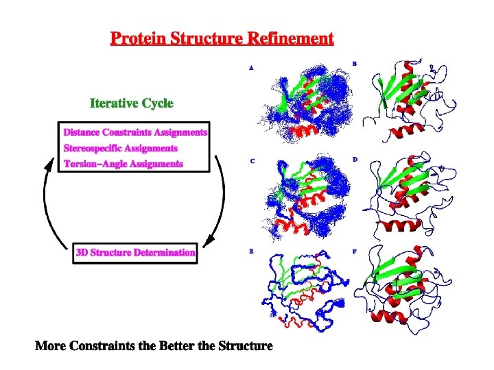
 Diagonal peaks are correlated by through-space Dipole-dipole interaction.")
2 D NOESY (Nuclear Overhauser Effect) Diagonal peaks are correlated by through-space Dipole-dipole interaction. NOE is a relaxation factor that builds-up during The “mixing-time (tm) The relative magnitude of the cross-peak is Related to the distance (1/r 6) between the Protons (≥ 5Ă). Basis for solving a Structure!

Protein NMR Number of atoms in a protein makes NMR spectra complex Resonance overlap Isotope label protein with 13 C and 15 N and spread spectra out in 3 D and 4 D

Protein NMR How do you assign a protein NMR spectra? A collection of “COSY”-like experiments that sequentially walk down the proteins’ backbone 3 D-NMR experiments that Require 13 C and 15 N labeled Protein sample Detect couplings to NH

Protein NMR Assignment strategy We know the primary sequence of the protein. Connect the overlapping correlation between NMR experiments

Protein NMR Molecular-weight Problem Higher molecular-weight –> more atoms –> more NMR resonance overlap More dramatic: NMR spectra deteriorate with increasing molecular-weight. MW increases -> correlation time increases -> T 2 decreases -> line-width increases NMR lines broaden to the point of not being detected! With broad lines, correlations (J, NOE) become less-efficient
 Deuterium label the protein. 1.")
Protein NMR How to Solve the Molecular-weight Problem? 1) Deuterium label the protein. 1. replace 1 H with 2 H and remove efficient relaxation paths 2. NMR resonances sharpen 3. problem: no hydrogens -> no NOEs -> no structure 4. actually get exchangeable (NH –NH) noes can 5. augment with specific 1 H labeling 1. 2) TROSY 1. line-width is field dependent
- Slides: 69