NRCSE Spacetime processes Spacetime processes Separable covariance structure

NRCSE Space-time processes

Space-time processes Separable covariance structure: Cov(Z(x, t), Z(y, s))=C 1(x, y)C 2(s, t) Nonseparable alternatives • Temporally varying spatial covariances • Fourier approach • Completely monotone functions

SARMAP revisited Spatial correlation structure depends on hour of the day:

Bruno’s seasonal nonseparability Nonseparability generated by seasonally changing spatial term Z 1 large-scale feature Z 2 separable field of local features (Bruno, 2004)

General stationary space-time covariances Cressie & Huang (1999): By Bochner’s theorem, a continuous, bounded, symmetric integrable C(h; u) is a spacetime covariance function iff is a covariance function for all w. Usage: Fourier transform of Cw(u) Problem: Need to know Fourier pairs

Spectral density Under stationarity and separability, If spatially nonstationary, write Define the spatial coherency as Under separability this is independent of frequency τ

Estimation Let where R is estimated using

Models-3 output

ANOVA results Item df rss P-value Between points 1 0. 129 0. 68 Between freqs 5 11. 14 0. 0008 Residual 5 0. 346

Coherence plot a 3, b 3 a 6, b 6

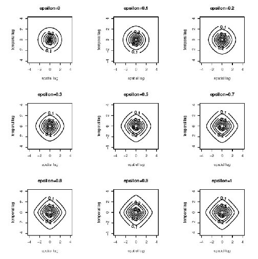
A class of Matérn-type nonseparable covariances scale spatial decay temporal decay space-time interaction =1: separable =0: time is space (at a different rate)

Chesapeake Bay wind field forecast (July 31, 2002)

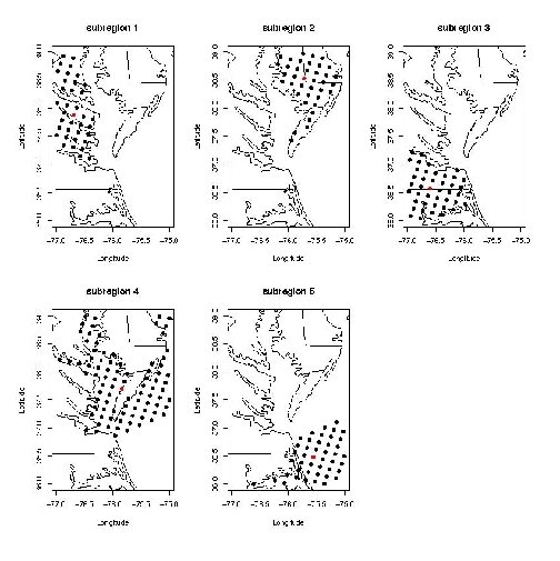
Fuentes model Prior equal weight on =0 and =1. Posterior: mass (essentially) 0 for =0 for regions 1, 2, 3, 5; mass 1 for region 4.

Another approach Gneiting (2001): A function f is completely monotone if (-1)nf(n)≥ 0 for all n. Bernstein’s theorem shows that for some nondecreasing F. In particular, is a spatial covariance function for all dimensions iff f is completely monotone. The idea is now to combine a completely monotone function and a function y with completey monotone derivative into a space-time covariance

Some examples

A particular case a=1/2, g=1/2 a=1/2, g=1 a=1, g=1/2 a=1, g=1

Issues to be developed • Nonstationarity Deformation approach: 3 -d spline fit; penalty for roughness in time and space • Antisymmetry Gneiting’s approach has C(h, u)=C(-h, u)=C(h, -u)=C(-h, -u) Unrealistic when covariance caused by meteorology • Covariates Need to take explicit account of covariates driving the covariance • Multivariate fields Mardia & Goodall (1992) use Kronecker product structure (like separability)

Temporally changing spatial deformations where

Velocity-driven space-time covariances CS covariance of purely spatial field V (random) velocity of field Space-time covariance Frozen field model: P(V=v)=1 (e. g. prevailing wind)

Taylor’s hypothesis C(0, u) = C(vu, 0) for some v Relates spatial to temporal covariance Examples: Frozen field model Separable models

Irish wind data Daily average wind speed at 11 stations, 1961 -70, transformed to “velocity measures” Spatial: exponential with nugget Temporal: Space-time: mixture of Gneiting model and frozen field

Evidence of asymmetry

Time lag 0 Time lag 1 Time lag 2 Time lag 3