Normalized Cuts and Image Segmentation Advanced Topics in

Normalized Cuts and Image Segmentation Advanced Topics in Computer Vision Amir Lev-Tov IDC, Herzliya

Main References Ø [1] Normalized Cuts and Image Segmentation, Shi and Malik, IEEE Conf. Computer Vision and Pattern Recognition, 1997. Ø [2] Normalized Cuts and Image Segmentation, Shi and Malik, IEEE Transactions on pattern analysis and machine intelligence, Vol 22, No 8, 2000

More References [3] Weiss Y. Segmentation using eigenvectors: a unifying view. Proceedings IEEE International Conference on Computer Vision, 1999. Ø [4] Ng A. Y. , Jordan , M. I. , and Weiss Y, On Spectral Clustering: Analysis and an algorithm, NIPS 2001 Ø [5] Rayleigh’s Quotient, Nail Gumerov, 2003 Ø [6] Wu and Leahy, an optimal graph theoretic approach to data clustering, PAMI, 1993 Ø

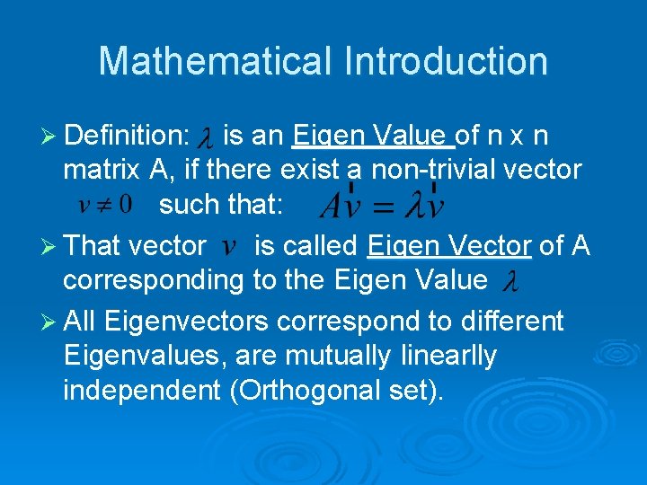
Mathematical Introduction Ø Definition: is an Eigen Value of n x n matrix A, if there exist a non-trivial vector such that: Ø That vector is called Eigen Vector of A corresponding to the Eigen Value Ø All Eigenvectors correspond to different Eigenvalues, are mutually linearlly independent (Orthogonal set).

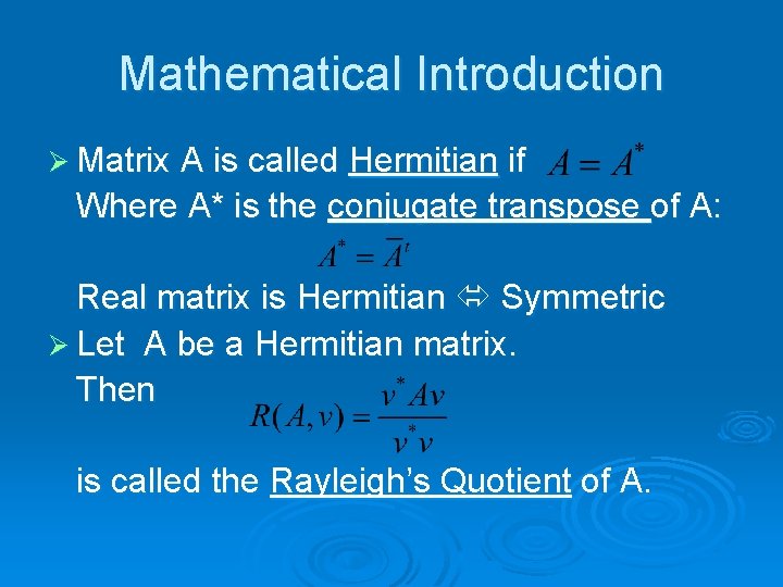
Mathematical Introduction Ø Matrix A is called Hermitian if Where A* is the conjugate transpose of A: Real matrix is Hermitian Symmetric Ø Let A be a Hermitian matrix. Then is called the Rayleigh’s Quotient of A.

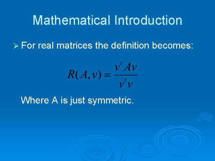
Mathematical Introduction Ø For real matrices the definition becomes: Where A is just symmetric.

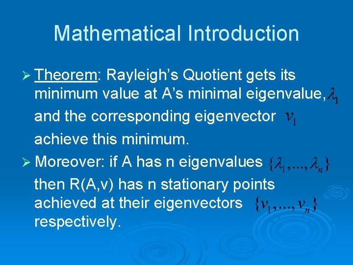
Mathematical Introduction Ø Theorem: Rayleigh’s Quotient gets its minimum value at A’s minimal eigenvalue, and the corresponding eigenvector achieve this minimum. Ø Moreover: if A has n eigenvalues then R(A, v) has n stationary points achieved at their eigenvectors respectively.

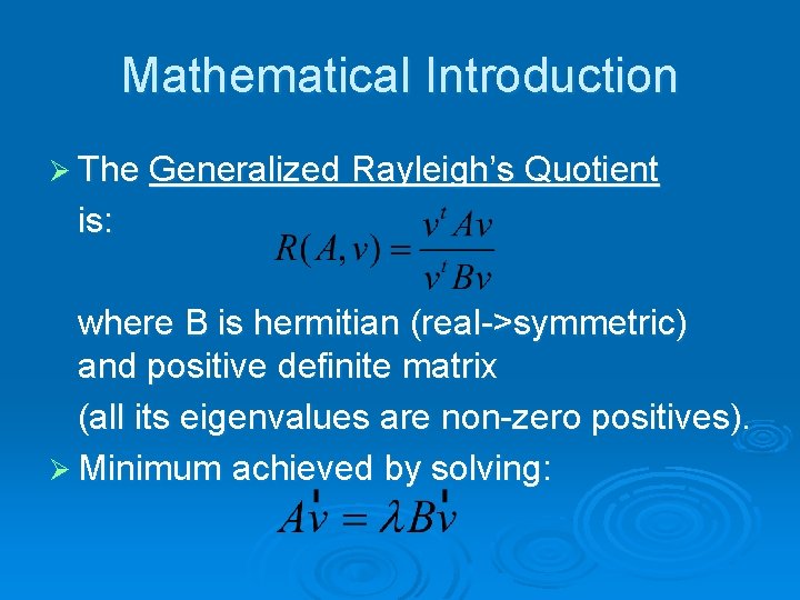
Mathematical Introduction Ø The Generalized Rayleigh’s Quotient is: where B is hermitian (real->symmetric) and positive definite matrix (all its eigenvalues are non-zero positives). Ø Minimum achieved by solving:

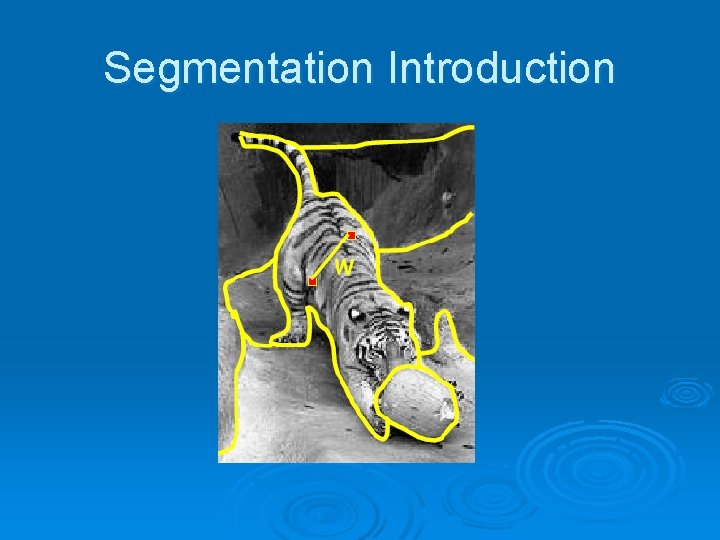
Segmentation Introduction

Segmentation Introduction Ø Problem: Divide an image into subsets of pixels (Segments). Ø Some methods: l l l Thresholding Region Growing K-means Mean-Shift Use of changes in color, texture etc. Contours

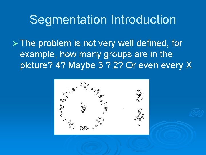
Segmentation Introduction Ø The problem is not very well defined, for example, how many groups are in the picture? 4? Maybe 3 ? 2? Or even every X

Segmentation Introduction Ø In order to get good Segmentation: l l Low level cues like colors, texutre etc. High level knowledge as global impression from the picture (top->down). Ø Need good similarity function Ø Number of segments is not known in advance

The Graph partitioning method Ø Main Idea: l l l Model the image by a graph G=(V, E). Assign similarity values to edges weights. Find a cut in G of minimal value, which yield partition of V into two subsets. • Matrix representation of computations. • Using Linear Algebra tools and Spectral Analysis to solve the new minimization problem. l Recursively repartition the subpartitions.

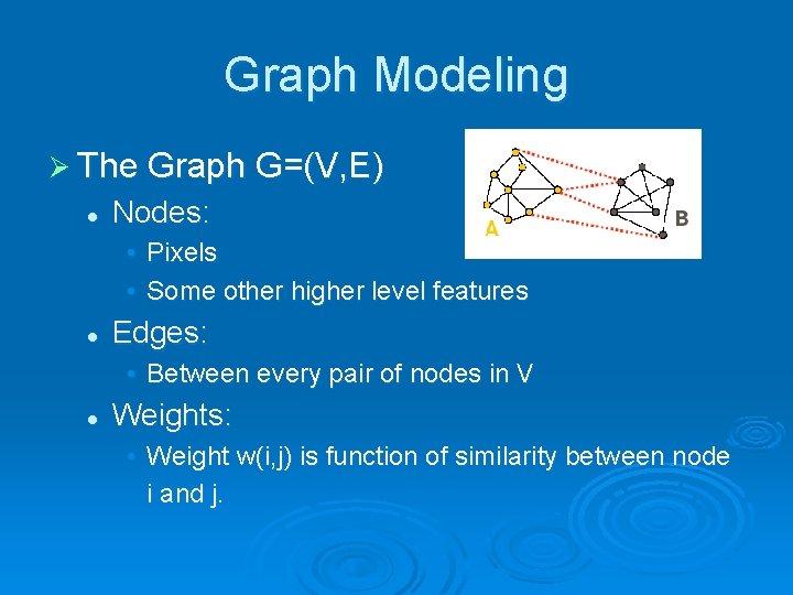
Graph Modeling Ø The Graph G=(V, E) l Nodes: • Pixels • Some other higher level features l Edges: • Between every pair of nodes in V l Weights: • Weight w(i, j) is function of similarity between node i and j.

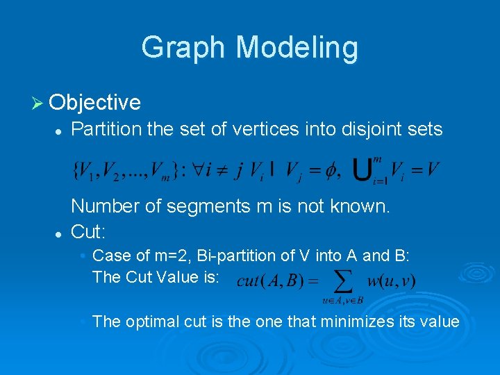
Graph Modeling Ø Objective l Partition the set of vertices into disjoint sets l Number of segments m is not known. Cut: • Case of m=2, Bi-partition of V into A and B: The Cut Value is: • The optimal cut is the one that minimizes its value

Minimun Cut Ø Wu and Leahy[1993]: l l Use the mentioned cut criteria Partition G into k subgraphs recursively Minimize the maximum cut value Produce good segmentation on some of the images

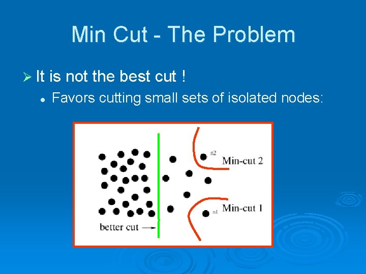
Min Cut - The Problem Ø It is not the best cut ! l Favors cutting small sets of isolated nodes:

Normalized Cut [Shi, Malick, 1997] Ø Normalize the cut value with the volume of the partition: Where

Normalized Cut Ø Properties: l l l Sets with weak connections Get low Ncut value. High Association within Sets Get low Ncut value. But - small sets are panalized with high Ncut value.

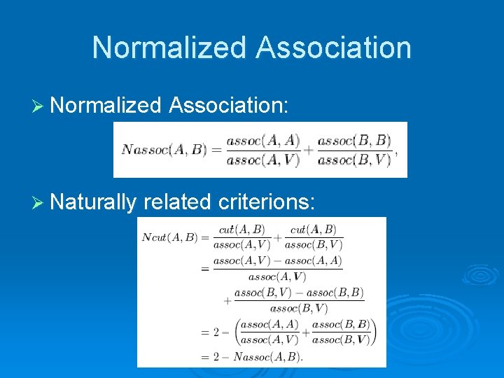
Normalized Association Ø Normalized Association: Ø Naturally related criterions:

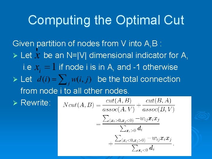
Computing the Optimal Cut Given partition of nodes from V into A, B : Ø Let be an N=|V| dimensional indicator for A, i. e if node i is in A, and -1 otherwise Ø Let be the total connection from node i to all other nodes. Ø Rewrite:

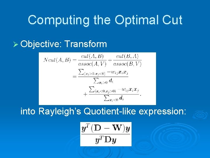
Computing the Optimal Cut Ø Objective: Transform into Rayleigh’s Quotient-like expression:

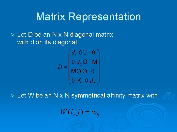
Matrix Representation Ø Let D be an N x N diagonal matrix with d on its diagonal: Ø Let W be an N x N symmetrical affinity matrix with

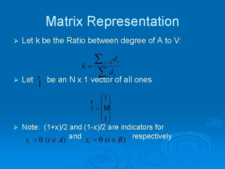
Matrix Representation Ø Let k be the Ratio between degree of A to V: Ø Let Ø Note: (1+x)/2 and (1 -x)/2 are indicators for and respectively be an N x 1 vector of all ones

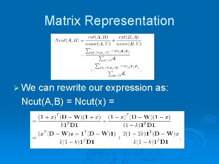
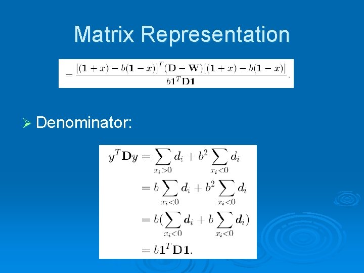
Matrix Representation Ø We can rewrite our expression as: Ncut(A, B) = Ncut(x) =

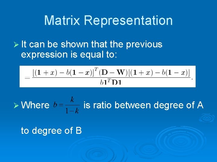
Matrix Representation Ø It can be shown that the previous expression is equal to: Ø Where to degree of B is ratio between degree of A

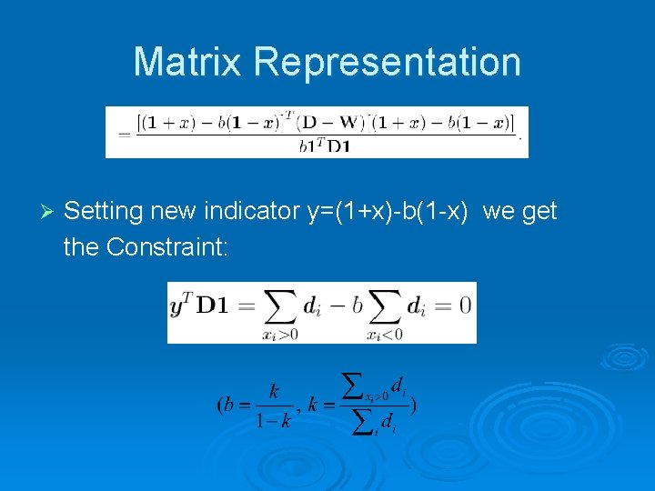
Matrix Representation Ø Setting new indicator y=(1+x)-b(1 -x) we get the Constraint:

Matrix Representation Ø Denominator:

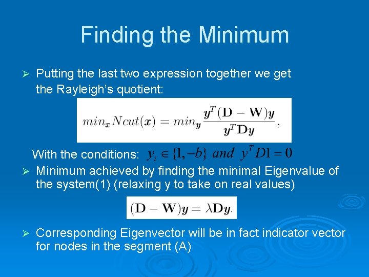
Finding the Minimum Ø Putting the last two expression together we get the Rayleigh’s quotient: With the conditions: Ø Minimum achieved by finding the minimal Eigenvalue of the system(1) (relaxing y to take on real values) Ø Corresponding Eigenvector will be in fact indicator vector for nodes in the segment (A)

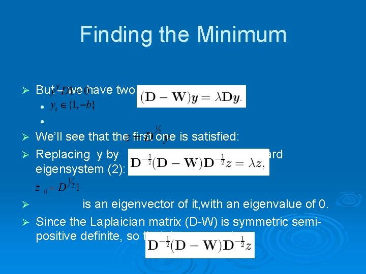
Finding the Minimum Ø But – we have two constraints: l l We’ll see that the first one is satisfied: Ø Replacing y by we get the standard eigensystem (2): Ø is an eigenvector of it, with an eigenvalue of 0. Ø Since the Laplaician matrix (D-W) is symmetric semipositive definite, so that the new system Ø

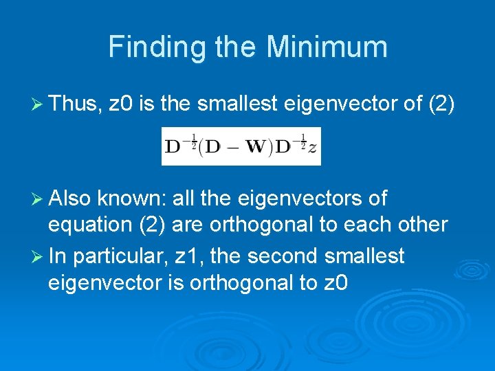
Finding the Minimum Ø Thus, z 0 is the smallest eigenvector of (2) Ø Also known: all the eigenvectors of equation (2) are orthogonal to each other Ø In particular, z 1, the second smallest eigenvector is orthogonal to z 0

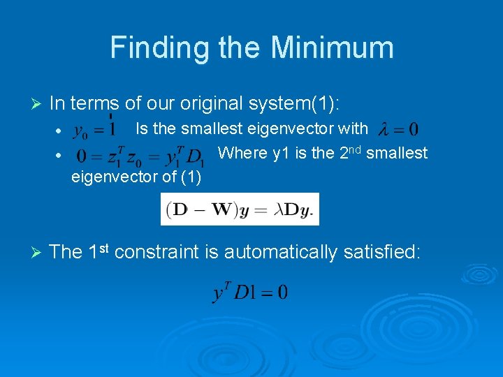
Finding the Minimum Ø In terms of our original system(1): l l Ø Is the smallest eigenvector with Where y 1 is the 2 nd smallest eigenvector of (1) The 1 st constraint is automatically satisfied:

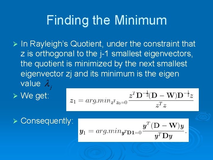
Finding the Minimum In Rayleigh’s Quotient, under the constraint that z is orthogonal to the j-1 smallest eigenvectors, the quotient is minimized by the next smallest eigenvector zj and its minimum is the eigen value Ø We get: Ø Ø Consequently:

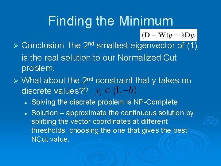
Finding the Minimum Conclusion: the 2 nd smallest eigenvector of (1) is the real solution to our Normalized Cut problem. Ø What about the 2 nd constraint that y takes on discrete values? ? Ø l l Solving the discrete problem is NP-Complete Solution – approximate the continuous solution by splitting the vector coordinates at different thresholds, choosing the one that gives the best NCut value.

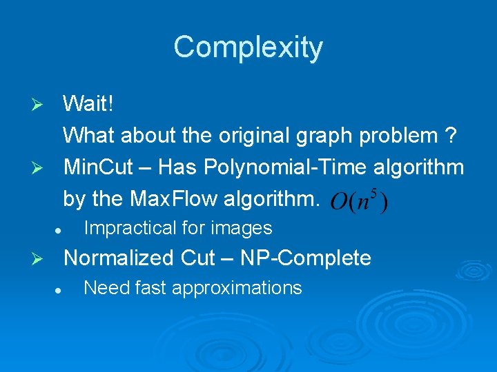
Complexity Wait! What about the original graph problem ? Ø Min. Cut – Has Polynomial-Time algorithm by the Max. Flow algorithm. Ø l Impractical for images Normalized Cut – NP-Complete Ø l Need fast approximations

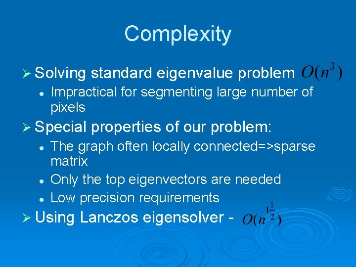
Complexity Ø Solving standard eigenvalue problem l Impractical for segmenting large number of pixels Ø Special properties of our problem: l l l The graph often locally connected=>sparse matrix Only the top eigenvectors are needed Low precision requirements Ø Using Lanczos eigensolver -

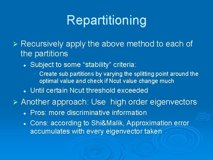
Repartitioning Ø Recursively apply the above method to each of the partitions l Subject to some “stability” criteria: • Create sub partitions by varying the splitting point around the optimal value and check if Ncut value change much l Ø Until certain Ncut threshold exceeded Another approach: Use high order eigenvectors l l Pros: more discriminative information Cons: according to Shi&Malik, Approximation error accumulates with every eigenvector taken

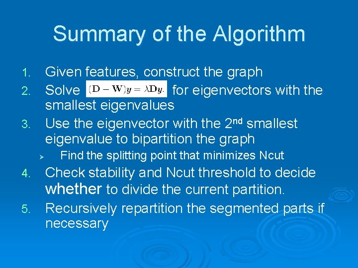
Summary of the Algorithm Given features, construct the graph 2. Solve for eigenvectors with the smallest eigenvalues 3. Use the eigenvector with the 2 nd smallest eigenvalue to bipartition the graph 1. Ø Find the splitting point that minimizes Ncut Check stability and Ncut threshold to decide whether to divide the current partition. 5. Recursively repartition the segmented parts if necessary 4.

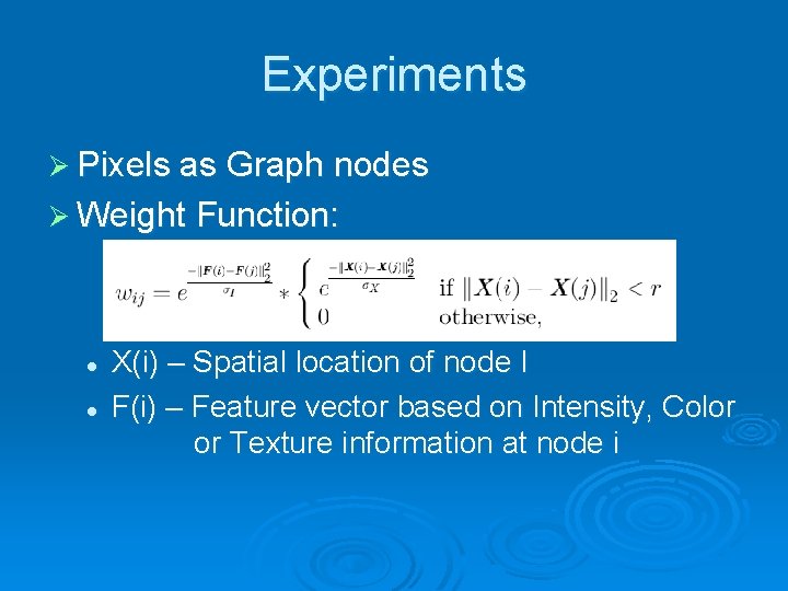
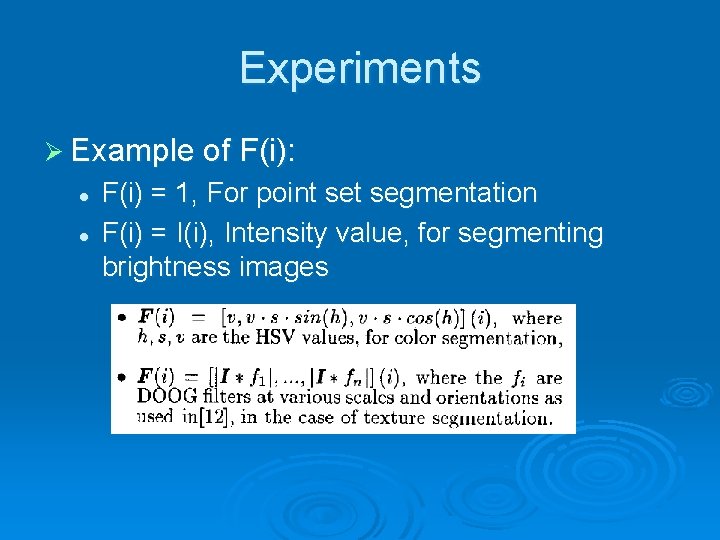
Experiments Ø Pixels as Graph nodes Ø Weight Function: l l X(i) – Spatial location of node I F(i) – Feature vector based on Intensity, Color or Texture information at node i

Experiments Ø Example of F(i): l l F(i) = 1, For point segmentation F(i) = I(i), Intensity value, for segmenting brightness images

Experiments Ø Point set Taken from [1]

Experiments Ø Synthetic image of corner Taken from [1]

Experiments Taken from [1]

Experiments Ø “Color” image Taken from [1]

Experiments Ø Without well defined boundaries: Taken from [1]

Experiments Ø Texture segmentation l Different orientation stripes Taken from [1]

. . A little bit more Taken from [2]

. . A little bit more Ø High order eigenvectors Taken from [2]

High order eigenvectors Taken from [2]

1 st Vs 2 nd Eigenvectors Taken from [3]

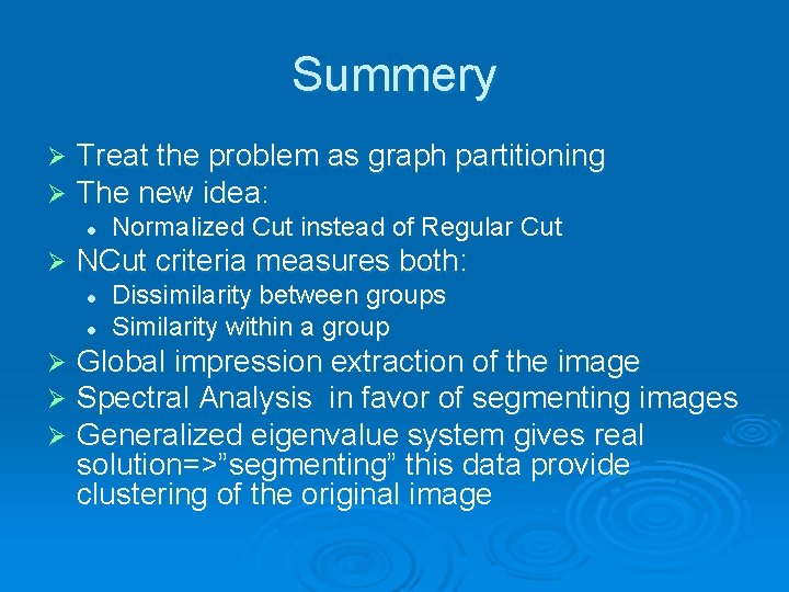
Summery Ø Ø Treat the problem as graph partitioning The new idea: l Ø NCut criteria measures both: l l Ø Ø Ø Normalized Cut instead of Regular Cut Dissimilarity between groups Similarity within a group Global impression extraction of the image Spectral Analysis in favor of segmenting images Generalized eigenvalue system gives real solution=>”segmenting” this data provide clustering of the original image

Thanks!