Normal Reference Range in Medicine and Skewed Distributions

Normal Reference Range in Medicine and Skewed Distributions Richard B. Goldstein, Ph. D. Professor of Mathematics (ret. ) Providence College Courtesy Professor of Mathematics at FGCU

Normal Reference Range : the set of values in which 95% of the normal population falls within (that is, a 95% prediction interval). It is determined by collecting data from typically over one hundred tests from normal patients.

Descriptive Statistics

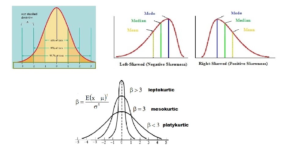
Common Methods used to calculate the Normal Reference Range • Sample mean ± 2 standard deviations • Percentiles of Raw Data • Using general power transformations to create a Normal/Gaussian Distribution • Curve fitting of data in histogram format by various skewed distributions • Dissecting distributions that contain mixed normal and abnormal populations

Near Gaussian Shaped Data

Some Raw Data – Creatinine (mg/dl) for 100 healthy males # Creatinine # Creatinine 1 0. 90 21 0. 97 41 1. 01 61 1. 04 81 1. 09 2 0. 91 22 0. 98 42 1. 01 62 1. 05 82 1. 09 3 0. 91 23 0. 98 43 1. 01 63 1. 05 83 1. 10 4 0. 92 24 0. 98 44 1. 01 64 1. 05 84 1. 10 5 0. 93 25 0. 98 45 1. 02 65 1. 05 85 1. 10 6 0. 93 26 0. 98 46 1. 02 66 1. 05 86 1. 10 7 0. 94 27 0. 99 47 1. 02 67 1. 06 87 1. 11 8 0. 94 28 0. 99 48 1. 02 68 1. 06 88 1. 11 9 0. 94 29 0. 99 49 1. 02 69 1. 06 89 1. 11 10 0. 95 30 0. 99 50 1. 03 70 1. 06 90 1. 12 11 0. 95 31 0. 99 51 1. 03 71 1. 07 91 1. 12 12 0. 96 32 1. 00 52 1. 03 72 1. 07 92 1. 13 13 0. 96 33 1. 00 53 1. 03 73 1. 07 93 1. 13 14 0. 96 34 1. 00 54 1. 03 74 1. 07 94 1. 13 15 0. 96 35 1. 00 55 1. 03 75 1. 08 95 1. 14 16 0. 97 36 1. 00 56 1. 03 76 1. 08 96 1. 15 17 0. 97 37 1. 00 57 1. 04 77 1. 08 97 1. 15 18 0. 97 38 1. 00 58 1. 04 78 1. 08 98 1. 16 19 0. 97 39 1. 00 59 1. 04 79 1. 09 99 1. 17 20 0. 97 40 1. 01 60 1. 04 80 1. 09 100 1. 19

The n sample values are used to find the sample statistics: Creatinine 20 18 16 14 12 10 8 6 4 2 0 0. 93 0. 96 0. 99 1. 02 1. 05 1. 08 1. 11 1. 14 1. 17 1. 2

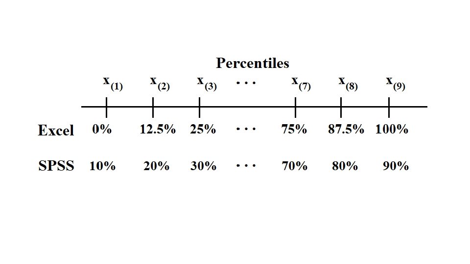
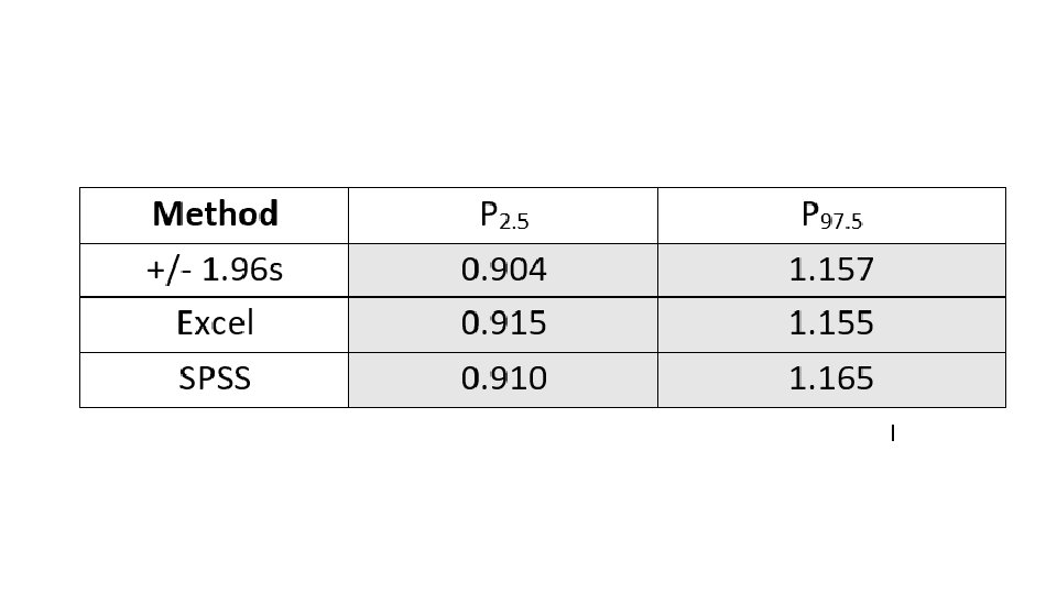
Using Percentiles on Raw Data The n sample values are sorted: Method I (used by Excel and Quattro Pro for example)

Method II (used by SPSS and known as Tukey’s Hinges) [a] [b] [c] if k(n + 1) < 1 then use r = 1 if k(n + 1) > n then use r = n otherwise interpolate using r = k(n + 1) Using this method the normal range is 0. 910 to 1. 165 The National Committee for Clinical Laboratory Standards accepted the use of percentiles as an optional method for determining a normal range which was proposed by L. Herrera.

ERRORS IN CLINICAL LABORATORIES • • Variations between laboratories Variation between analysts (same laboratory site) Day-to-day variations (same analyst, laboratory, and sample) Variations between replicates (same analysis) 2. 0 SD 1. 0 SD 20 20 15 15 15 10 5 0 0. 75 0. 80 0. 85 0. 90 0. 95 1. 00 1. 05 Creatinine mg/dl 1. 10 1. 15 1. 20 1. 25 Frequency 20 Frequency 0. 5 SD 10 5 5 0 0 0. 75 10 0. 85 0. 90 0. 95 1. 00 1. 05 Creatinine mg/dl 1. 10 1. 15 1. 20 1. 25 0. 75 0. 80 0. 85 0. 90 0. 95 1. 00 1. 05 Creatinine mg/dl 1. 10 1. 15 1. 20 1. 25

CONVOLUTION (sum of random variables) Z = X + Y X has probability density function f(x) Y has probability density function g(x) Z has probability density function h(x) Example: Exponential and Normal Distributions

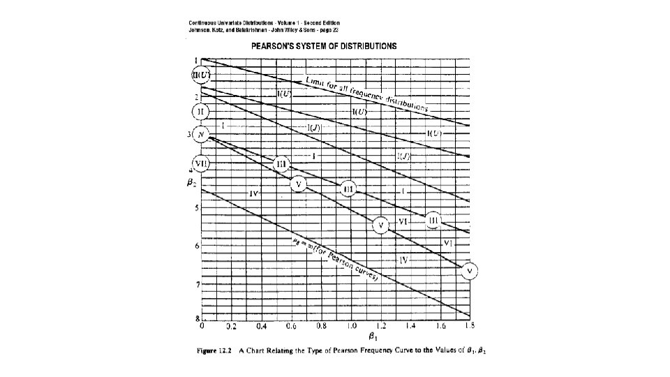
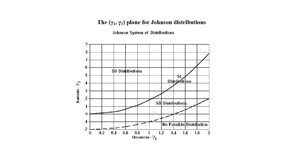
Skewed Distributions for Fitting Data • Gram – Charlier Series • Pearson System of Distributions • N. L. Johnson System of Distributions • Skew-Normal Distribution

Gram-Charlier Series Problems: 1. f(x) is negative for part of the interval 2. f(x) is bimodal for high skewness

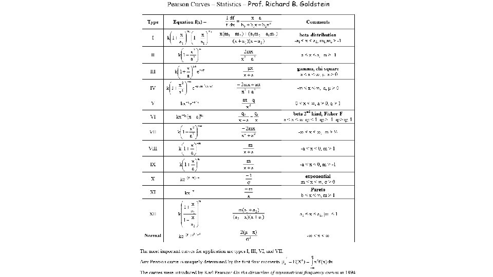
Karl Pearson System of Distributions Problems: 1. Difficulty in finding percentiles 2. Some complicated forms

N. L. Johnson System of Probability Distributions

Highly Skewed Distribution – A 1 c/Glycated Hemoglobin x 3. 25 3. 75 4. 25 4. 75 5. 25 5. 75 6. 25 6. 75 7. 25 7. 75 8. 25 8. 75 9. 25 9. 75 10. 25 10. 75 11. 25 11. 75 12. 25 12. 75 freq 1 5 17 110 183 102 23 10 4 4 2 2 1 3 0 1 1 A 1 c - Histogram of n = 474 in NHANES III Study 200 180 160 140 120 100 80 60 40 20 0 TOTAL 474 3. 25 3. 75 4. 25 4. 75 5. 25 5. 75 6. 25 6. 75 7. 25 7. 75 8. 25 8. 75 9. 25 9. 75 10. 25 10. 75 11. 25 11. 75 12. 25 12. 75

Sum Sq = 175. 4 P 0. 95 = 6. 06 First Fit A 1 c fit by Johnson SU 200 180 Standard: 4% to 5. 6% : Normal 5. 7% to 6. 4% : Pre-Diabetic 6. 5% or more : Diabetic 160 140 120 100 80 60 40 20 0 3. 25 3. 75 4. 25 4. 75 5. 25 5. 75 6. 25 6. 75 7. 25 7. 75 8. 25 8. 75 9. 25 9. 75 10. 25 10. 75 11. 25 11. 75 12. 25 12. 75 freq fit

Was this a set of healthy individuals only? Can we remove some abnormals/unhealthy? A 1 c - fit by Dissection by Johnson SU & Normal Distributions 200 180 160 140 120 100 80 60 40 20 0 0 0. 5 1 1. 5 2 2. 5 3 3. 5 4 4. 5 5 5. 5 6 SU-Normals 6. 5 7 7. 5 Gauss-Abnormal 8 8. 5 9 9. 5 10 10. 5 11 11. 5 12 12. 5 13 13. 5

Dissected result using Johnson SU & Gaussian • • • Dissection f. Tot (x)= w 1 f 1(x) + w 2 f 2(x) Sum of squares now 56. 71 Approximately 89% of values are healthy (normal) individuals Approximately 11% of values are from unhealthy (abnormal) individuals The 90 th percentile is 5. 82 The 95 th percentile is 5. 98 Standard (from sources): 4% to 5. 6% : Normal 5. 7% to 6. 4% : Pre-Diabetic 6. 5% or more : Diabetic

Dissection using two Johnson SU distributions 200 190 180 170 160 150 140 130 120 110 100 90 80 70 60 50 40 30 20 10 0 0 0. 5 1 1. 5 2 2. 5 3 3. 5 4 4. 5 5 Normal 5. 5 6 6. 5 Abnormal 7 7. 5 8 8. 5 9 9. 5 10 10. 5 11 11. 5 12 12. 5 13 13. 5

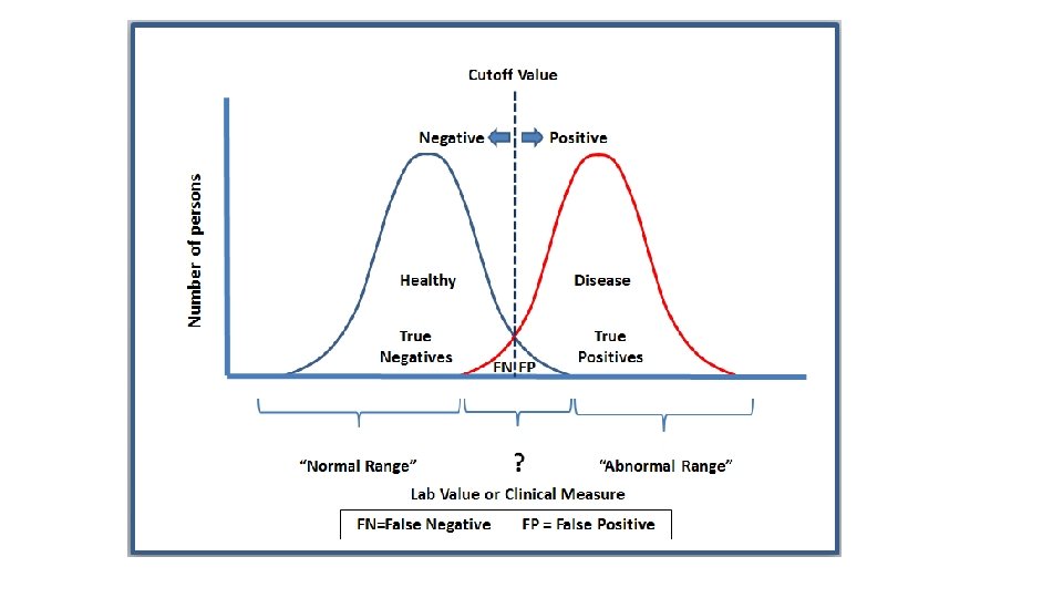
Dissected result using 2 Johnson SU Distributions • Sum of squares now 37. 73 • Approximately 91% of values are healthy individuals • Approximately 9% of values are from unhealthy individuals • The 90 th percentile is 5. 82 • The 95 th percentile is 5. 99 • Almost identical to using Johnson SU with Gaussian • Note crossover at 6. 4 where we minimize the sum of the false positives and false negatives

Comparisons for A 1 c Method Simple Normal +1. 645 s Single Johnson SU fit Dissection Johnson SU & Gauss Sum of Sqs Dissection 2 Johnson SU Current Standard Prediabetic Current Standard Diabetic 37. 7 175. 4 56. 7 95 th Percentile 7. 25 6. 06 5. 98 5. 99 5. 60 6. 50

Highly Skewed Data with Outliers

Some Raw Data – Lactate Dehydrogenase (IU/L) – Female Children

Box-Cox Transformation One way to determine, λ is to select the value of λ that maximizes the logarithm of the likelihood function (LLF):

LDH 119 - no transform 30 25 20 15 10 5 0 300 400 500 600 700 800 900 1000 1100 1200 1300 1400 1500 1600 1700 1800 1900 2000 2100 2200 2300 2400 2500 2600 2700 LDH 119 – after transform 8 = -0. 9742 25 20 15 10 5 0 1. 0229 1. 0232 1. 0235 1. 0238 1. 0241 1. 0244 1. 0247 1. 0250 1. 0253 1. 0256 1. 0259 1. 0262

OUTLIERS in a Normal Distrubtion Prof. John Tukey’s Exploratory Data Analysis First Fence beyond [Q 1 -1. 5*IQR] = -2. 698 or [Q 3+1. 5*IQR] = 2. 698 about 0. 698% totally – use symbol о Second Fence beyond [Q 1 -3*IQR] = -4. 721 or [Q 3+3*IQR] = 4. 721 about 0. 00023% totally – use symbol Ж For LDH where the 1 st fence is 1287. 6 and 2 nd fence is 1761. 2 there are 9 outliers of which 4 are extreme outliers – this is too many!

Outliers using John W. Tukey’s Box Plot

Outliers for a lognormal distribution • Here Q 1 = 0. 509, Q 3 = 1. 963 and the 1 st fence is 4. 143 and 2 nd is 6. 329. Using Tukey’s fences 7. 76% of the values are beyond the 1 st fence and 3. 26% are beyond 2 nd fence. • For LDH if the top 2 values (4537 and 66592) are dropped, then the 1 st fence is at 2873 and there would be no further outliers to remove. An outlier should be errors in measurement or extremely unlikely events. • Conclusion: Don’t use Tukey’s fences for very skewed data. • Suggestion: Transform data closer to Normal and then use Tukey’s fences to remove outliers.

LDH - Johnson SU 30 30 25 25 20 20 15 15 10 10 5 5 0 250 350 450 550 650 750 850 950 1050 1150 1250 1350 1450 1550 0 P 2. 5 = 375 P 97. 5 = 1432 Note: 4 values not fitted are 2327, 2614, 4537, and 66592

Comparisons for LDH Method Nonparametric 95% Reference Interval with all 120 LDH values (376, 2334) 95% Reference Interval with 116 LDH values (375, 1370) Traditional Normal Transformed Normal (0, 13271) (351, 1730) (194, 1138) (366, 1351) Least Sq fit by Johnson SU (305, 1104) (375, 1432) Traditional Normal: LDH Data Source: Reference Intervals: A User’s Guide by Horn & Pesce – AACC Press 2005

Cholesterol Data from the Framingham (MA) Heart Study # 1 2 3 4 5 6 7 8 9 10 11 12 13 14 15 16 Chol 167 184 192 198 200 202 210 211 212 215 216 217 218 220 225 # 17 18 19 20 21 22 23 24 25 26 27 28 29 30 31 32 Chol 226 230 230 231 232 232 234 236 238 240 243 # 33 34 35 36 37 38 39 40 41 42 43 44 45 46 47 48 Chol 246 247 248 254 254 256 258 263 264 267 267 268 270 # 49 50 51 52 53 54 55 56 57 58 59 60 61 62 Chol 270 272 278 283 285 300 308 327 334 336 353 393

The Heart Study began in 1948 by recruiting an Original Cohort of 5, 209 men and women between the ages of 30 and 62 from the town of Framingham, Massachusetts, who had not yet developed overt symptoms of cardiovascular disease or suffered a heart attack or stroke. Assuming the above data came from healthy individuals then p 95 = 334. This is way above current standards: Total Cholesterol Level Category Less than 200 MG/DL Desirable 200 -239 MG/DL Borderline High 240 MG/DL and above High

Tests for Normality Tests to Consider [1] Chi-Square Goodness-of-Fit Test [2] Graphics – Normal Probability Plot [3] Non-Parametric Kolmogorov-Smirnov Test [4] Geary’s Test for Normal Distribution [5] D’Agostino-Belanger-Pearson’s Skewness, Kurtosis, and Omnibus Tests [6] Others – Shapiro-Wilk, Anderson-Darling, Cramér-von Mises Tests

Other considerations • Use of powers and other transforms • Other distributions • Fitting by first 4 moments (Pearson system) vs. Least Squares • Confidence Intervals for predictions • Jackknife method or Resampling/Bootstrapping to get confidence intervals

Mathematicians who contributed Karl Friedrich Gauss Joseph Gram Carl Charlier Karl Pearson William S. Gosset (Student) Norman Lloyd Johnson George Box David Cox John W. Tukey 1777 -1855 1850 -1916 1862 -1934 1857 -1936 1876 -1937 1917 -2004 1919 -2000 19241915 -2000 Germany Denmark Sweden UK UK UK/USA

Dedicated to Prof. Horace F. Martin 1931 -2010 B. S. M. S. Ph. D. M. D. J. D. M. P. H. - Providence College 1953 - University of Rhode Island 1955 - Boston University 1961 - Brown University 1975 - S. New England Sch. of Law 1990 - Mc. Gill University 2000 44

Thank You Florida Gulf Coast University 45