normal form games with complete information part 2

normal form games with complete information part 2

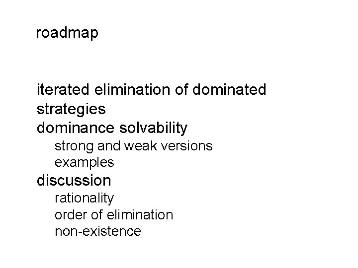
roadmap iterated elimination of dominated strategies dominance solvability strong and weak versions examples discussion rationality order of elimination non-existence

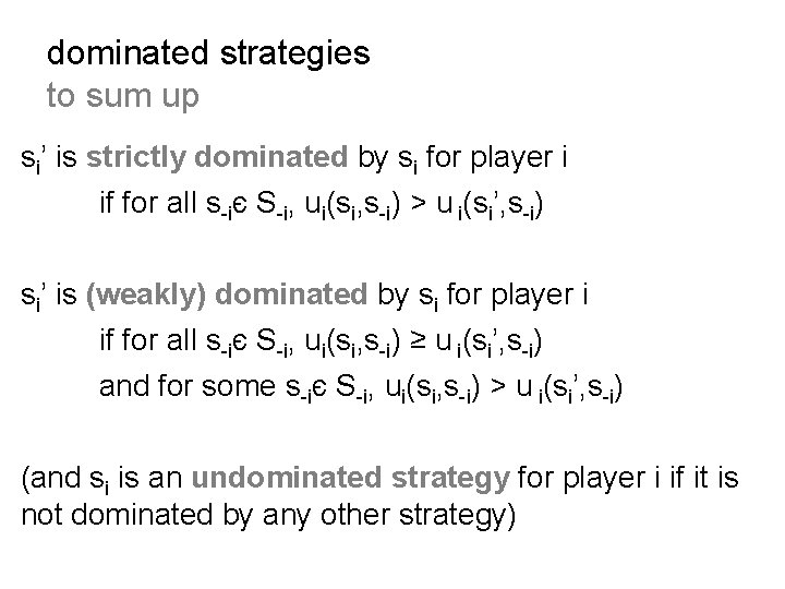
dominated strategies to sum up si’ is strictly dominated by si for player i if for all s-iє S-i, ui(si, s-i) > u i(si’, s-i) si’ is (weakly) dominated by si for player i if for all s-iє S-i, ui(si, s-i) ≥ u i(si’, s-i) and for some s-iє S-i, ui(si, s-i) > u i(si’, s-i) (and si is an undominated strategy for player i if it is not dominated by any other strategy)

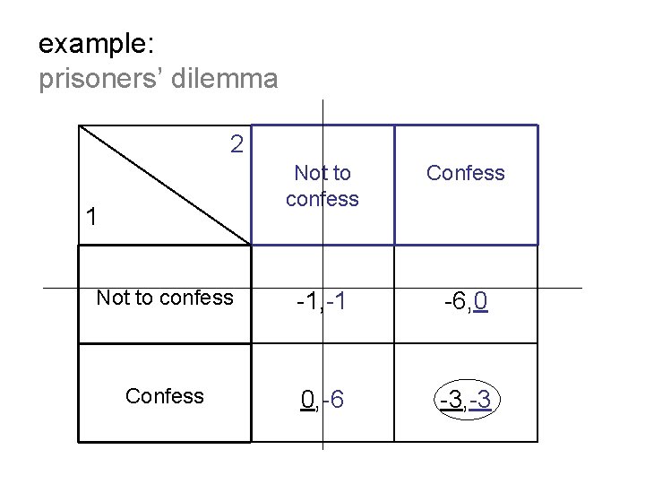
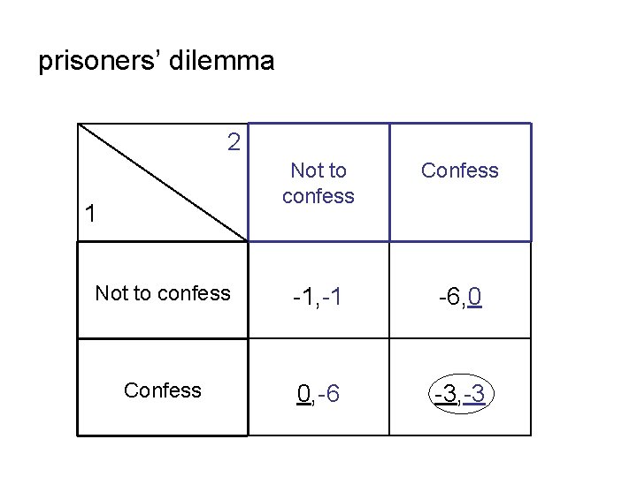
example: prisoners’ dilemma 2 Not to confess Confess Not to confess -1, -1 -6, 0 Confess 0, -6 -3, -3 1

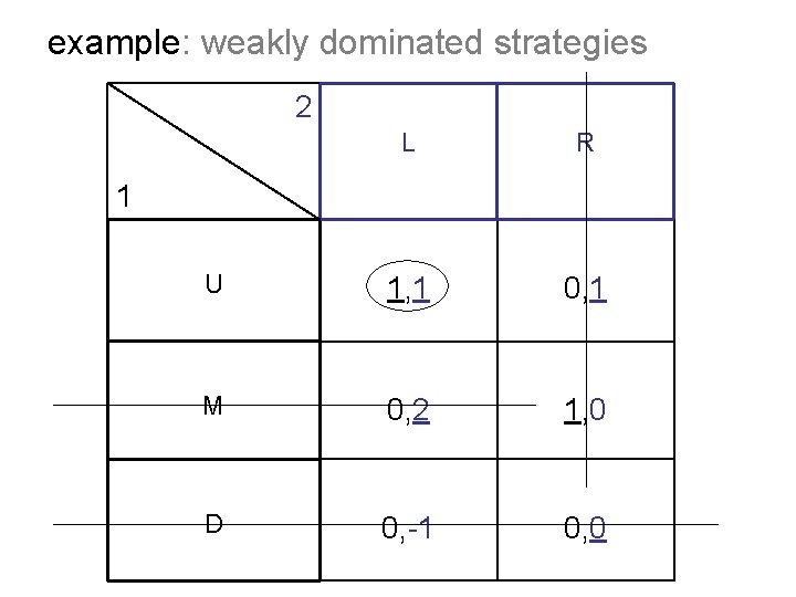
example: weakly dominated strategies 2 L R U 1, 1 0, 1 M 0, 2 1, 0 D 0, -1 0, 0 1

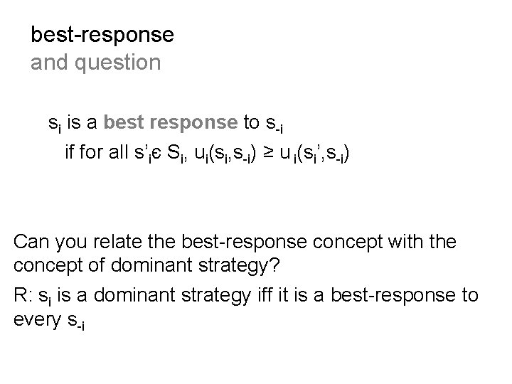
best-response and question si is a best response to s-i if for all s’iє Si, ui(si, s-i) ≥ u i(si’, s-i) Can you relate the best-response concept with the concept of dominant strategy? R: si is a dominant strategy iff it is a best-response to every s-i

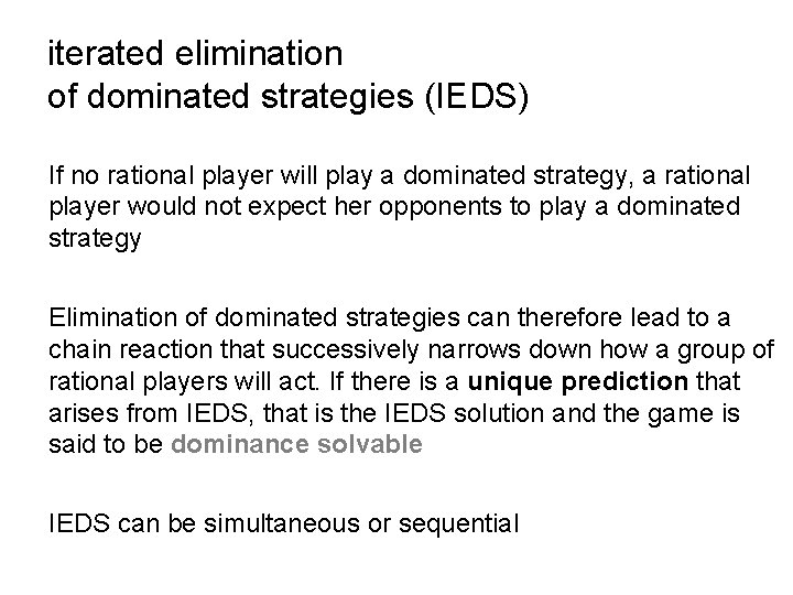
iterated elimination of dominated strategies (IEDS) If no rational player will play a dominated strategy, a rational player would not expect her opponents to play a dominated strategy Elimination of dominated strategies can therefore lead to a chain reaction that successively narrows down how a group of rational players will act. If there is a unique prediction that arises from IEDS, that is the IEDS solution and the game is said to be dominance solvable IEDS can be simultaneous or sequential

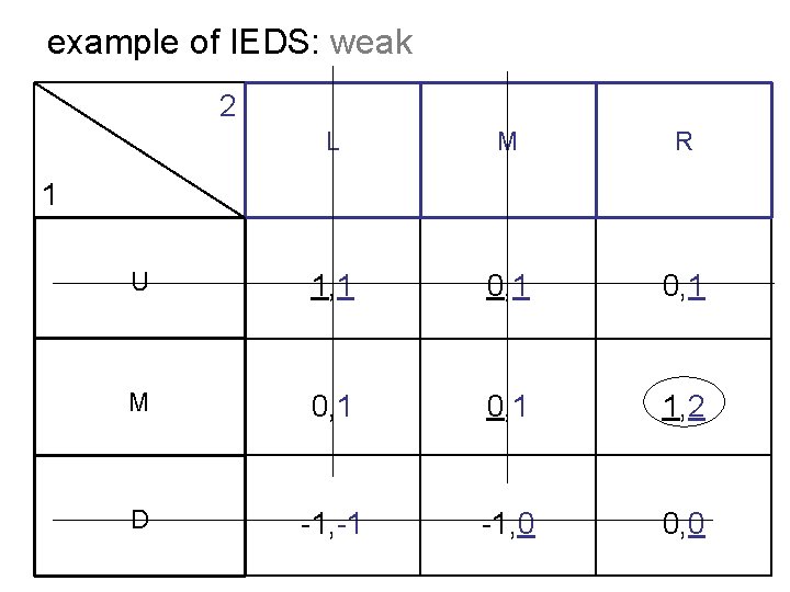
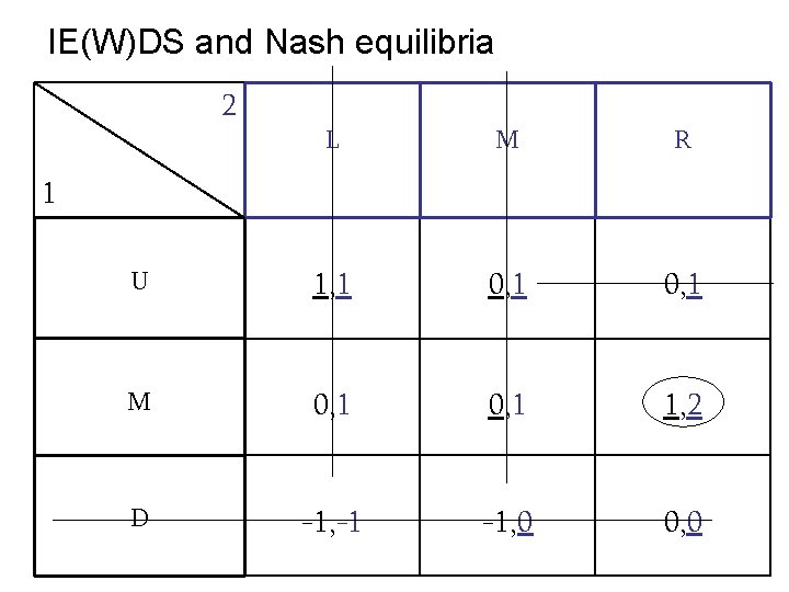
example of IEDS: weak 2 L M R U 1, 1 0, 1 M 0, 1 1, 2 D -1, -1 -1, 0 0, 0 1

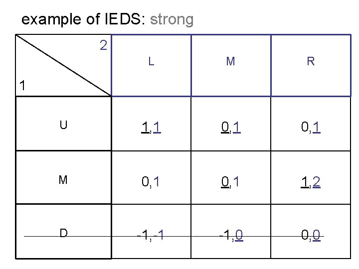
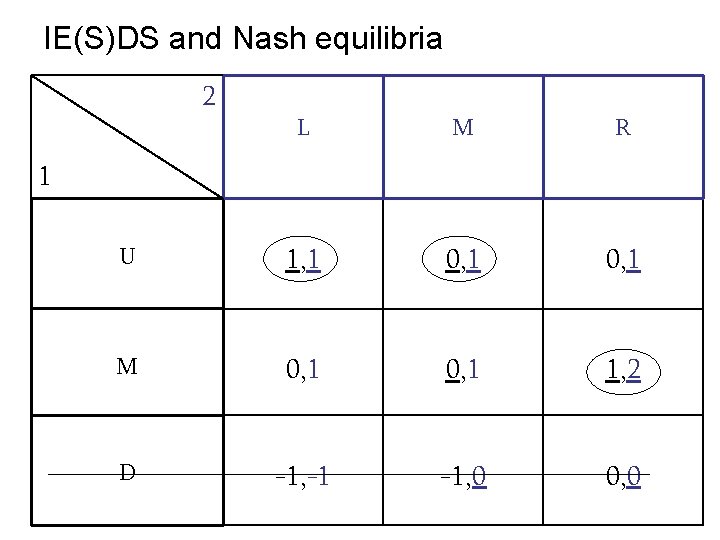
example of IEDS: strong 2 L M R U 1, 1 0, 1 M 0, 1 1, 2 D -1, -1 -1, 0 0, 0 1

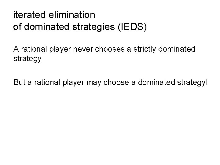
iterated elimination of dominated strategies (IEDS) A rational player never chooses a strictly dominated strategy But a rational player may choose a dominated strategy!

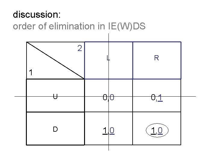
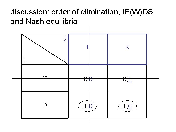
discussion: order of elimination in IE(W)DS 2 L R U 0, 0 0, 1 D 1, 0 1

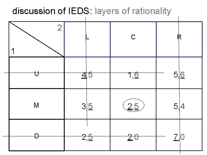
discussion of IEDS: layers of rationality 2 L C R U 4, 5 1, 6 5, 6 M 3, 5 2, 5 5, 4 D 2, 5 2, 0 7, 0 1

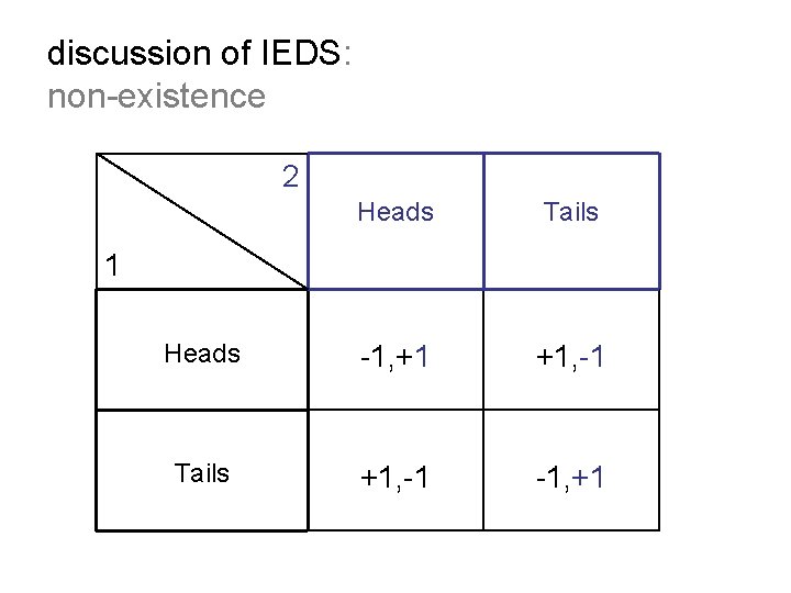
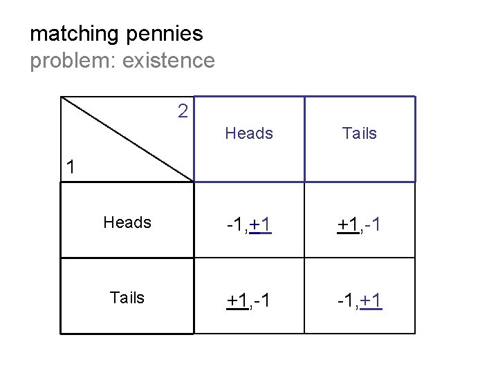
discussion of IEDS: non-existence 2 Heads Tails Heads -1, +1 +1, -1 Tails +1, -1 -1, +1 1

example 1 (homework) Each player i of n players selects a number xi between 0 and 100 simultaneously. Player i’s payoff is ui = xi-3 y/5, where y denotes the average of all numbers chosen

example 1 (homework) Normal form representation Is there any dominated strategy? What numbers should be selected?

example 2 (homework) Two players (1 and 2) are bidding at a painting’s auction. Their valuations (represented by vi) (willingness to pay) are common knowledge and are such that v 1 > v 2. The auction format is as follows. Each player i (simultaneously) submits a non-negative bid xi in a closed envelope. The auctioneer opens the envelopes. The highest bidder wins the auction and pays the other bidder’s bid. In case of a tie, bidder 1 wins the auction and pays the bid.

example 2 (homework) Normal form representation Is there any dominated strategy? What bids should be selected?

more homework: exercises 1 and 2

normal form games with complete information part 3

roadmap Nash equilibrium definition interpretations examples relation between Nash equilibrium and IEDS references Sec 1. 1. C and 1. 2. A, B of Gibbons Sec 2. 6 -2. 8 of Osborne Ch 5 of Dutta

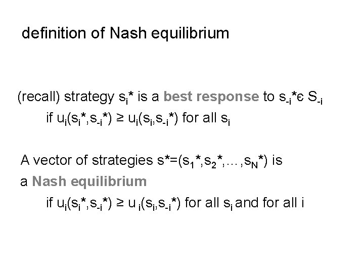
definition of Nash equilibrium (recall) strategy si* is a best response to s-i*є S-i if ui(si*, s-i*) ≥ ui(si, s-i*) for all si A vector of strategies s*=(s 1*, s 2*, …, s. N*) is a Nash equilibrium if ui(si*, s-i*) ≥ u i(si, s-i*) for all si and for all i

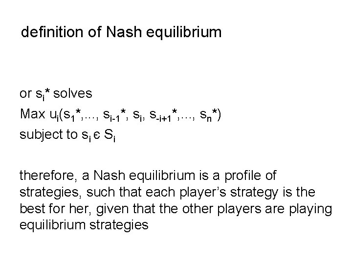
definition of Nash equilibrium or si* solves Max ui(s 1*, . . . , si-1*, si, s-i+1*, . . . , sn*) subject to si є Si therefore, a Nash equilibrium is a profile of strategies, such that each player’s strategy is the best for her, given that the other players are playing equilibrium strategies

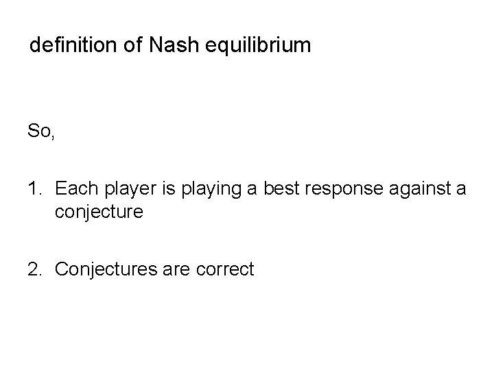
definition of Nash equilibrium So, 1. Each player is playing a best response against a conjecture 2. Conjectures are correct

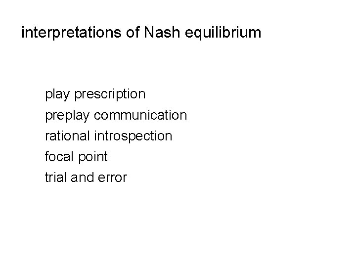
interpretations of Nash equilibrium play prescription preplay communication rational introspection focal point trial and error

prisoners’ dilemma 2 Not to confess Confess Not to confess -1, -1 -6, 0 Confess 0, -6 -3, -3 1

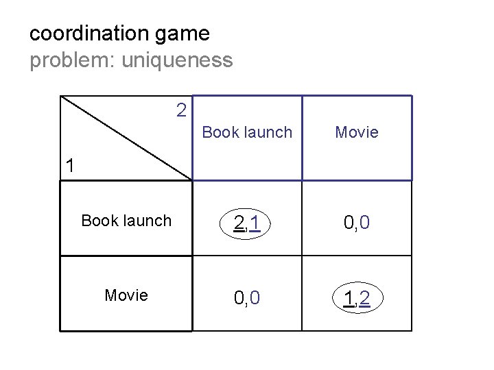
coordination game problem: uniqueness 2 Book launch Movie Book launch 2, 1 0, 0 Movie 0, 0 1, 2 1

matching pennies problem: existence 2 Heads Tails Heads -1, +1 +1, -1 Tails +1, -1 -1, +1 1

IE(W)DS and Nash equilibria 2 L M R U 1, 1 0, 1 M 0, 1 1, 2 D -1, -1 -1, 0 0, 0 1

IE(S)DS and Nash equilibria 2 L M R U 1, 1 0, 1 M 0, 1 1, 2 D -1, -1 -1, 0 0, 0 1

discussion: order of elimination, IE(W)DS and Nash equilibria 2 L R U 0, 0 0, 1 D 1, 0 1

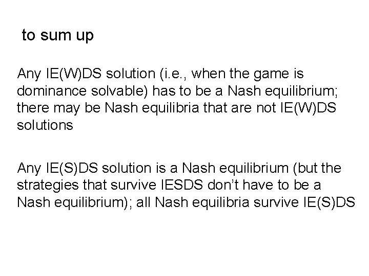
to sum up Any IE(W)DS solution (i. e. , when the game is dominance solvable) has to be a Nash equilibrium; there may be Nash equilibria that are not IE(W)DS solutions Any IE(S)DS solution is a Nash equilibrium (but the strategies that survive IESDS don’t have to be a Nash equilibrium); all Nash equilibria survive IE(S)DS

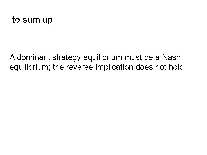
to sum up A dominant strategy equilibrium must be a Nash equilibrium; the reverse implication does not hold

normal form games with complete information part 4

roadmap solving a maximization problem Cournot model Bertrand models (with differentiated and homogeneous products) contributing to a public good references Sec 1. 2. B of Gibbons and Sec 3. 1 and 3. 2 of Osborne Ch 6 of Dutta

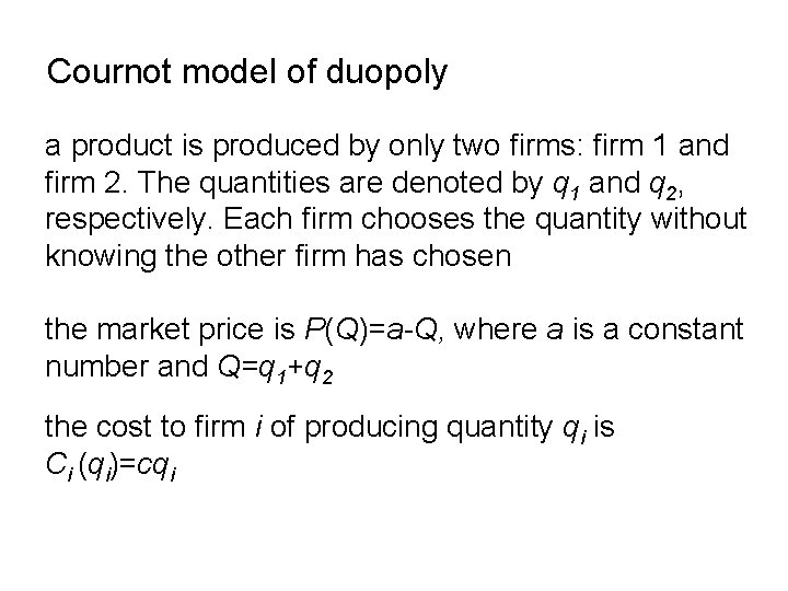
Cournot model of duopoly a product is produced by only two firms: firm 1 and firm 2. The quantities are denoted by q 1 and q 2, respectively. Each firm chooses the quantity without knowing the other firm has chosen the market price is P(Q)=a-Q, where a is a constant number and Q=q 1+q 2 the cost to firm i of producing quantity qi is Ci (qi)=cqi

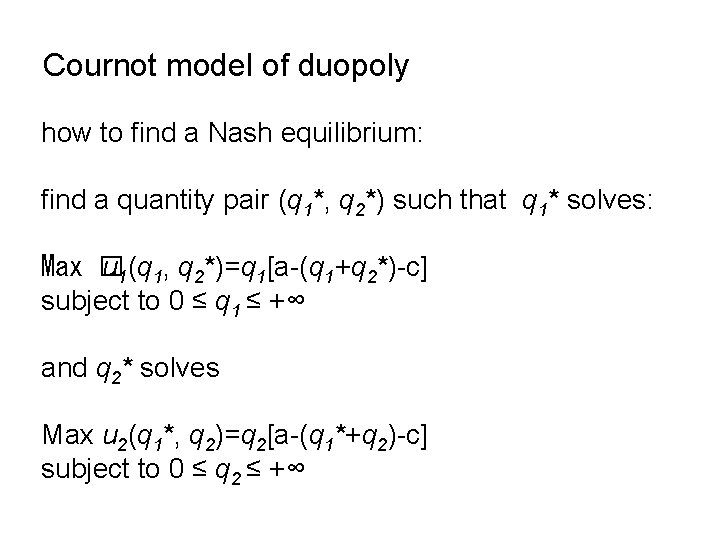
Cournot model of duopoly how to find a Nash equilibrium: find a quantity pair (q 1*, q 2*) such that q 1* solves: Max � u 1(q 1, q 2*)=q 1[a-(q 1+q 2*)-c] subject to 0 ≤ q 1 ≤ +∞ and q 2* solves Max u 2(q 1*, q 2)=q 2[a-(q 1*+q 2)-c] subject to 0 ≤ q 2 ≤ +∞

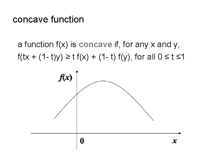
concave function a function f(x) is concave if, for any x and y, f(tx + (1 - t)y) ≥ t f(x) + (1 - t) f(y), for all 0 ≤ t ≤ 1

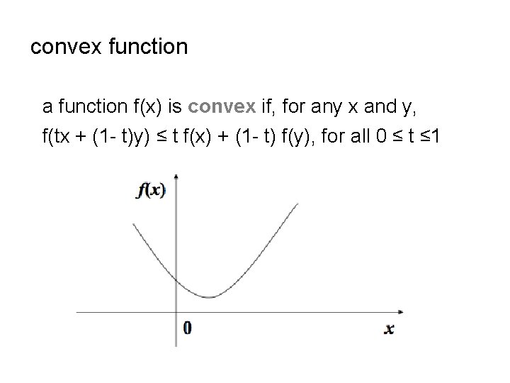
convex function a function f(x) is convex if, for any x and y, f(tx + (1 - t)y) ≤ t f(x) + (1 - t) f(y), for all 0 ≤ t ≤ 1

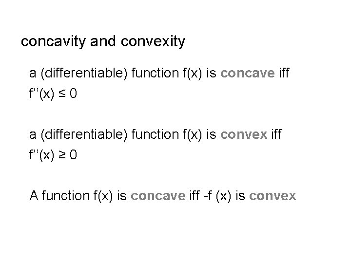
concavity and convexity a (differentiable) function f(x) is concave iff f’’(x) ≤ 0 a (differentiable) function f(x) is convex iff f’’(x) ≥ 0 A function f(x) is concave iff -f (x) is convex

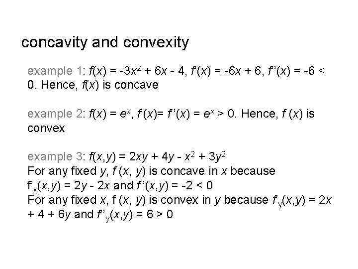
concavity and convexity example 1: f(x) = -3 x 2 + 6 x - 4, f’(x) = -6 x + 6, f’’(x) = -6 < 0. Hence, f(x) is concave example 2: f(x) = ex, f’(x)= f’’(x) = ex > 0. Hence, f (x) is convex example 3: f(x, y) = 2 xy + 4 y - x 2 + 3 y 2 For any fixed y, f (x, y) is concave in x because f’x(x, y) = 2 y - 2 x and f’’(x, y) = -2 < 0 For any fixed x, f (x, y) is convex in y because f’y(x, y) = 2 x + 4 + 6 y and f’’y(x, y) = 6 > 0

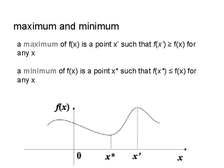
maximum and minimum a maximum of f(x) is a point x’ such that f(x’) ≥ f(x) for any x a minimum of f(x) is a point x* such that f(x*) ≤ f(x) for any x

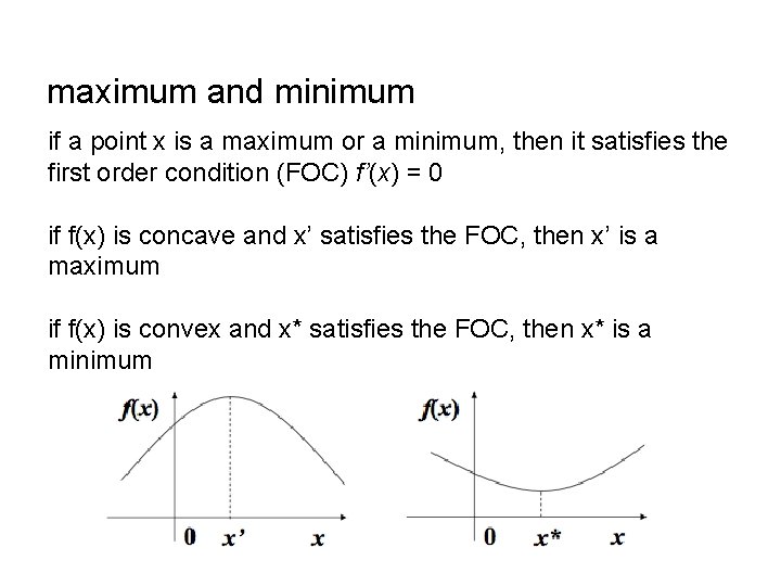
maximum and minimum if a point x is a maximum or a minimum, then it satisfies the first order condition (FOC) f’(x) = 0 if f(x) is concave and x’ satisfies the FOC, then x’ is a maximum if f(x) is convex and x* satisfies the FOC, then x* is a minimum

maximum and minimum a maximum of f(x) in the domain [x 1, x 2] is a point x’ in [x 1, x 2] such that f(x’) ≥ f(x) for all x € [x 1, x 2] a minimum of f(x) in the domain [x 1, x 2] is a point x* in [x 1, x 2] such that f(x*) ≤ f(x) for all x € [x 1, x 2]

finding a maximum of a concave function in [x 1, x 2] find a maximum x’ of f(x) without constraints if x’ is in [x 1, x 2] , then x’ is also a maximum for the constrained problem otherwise, a. if f(x 1) > f( x 2) or x’ < x 1, then x 1 is a maximum b. if f(x 1) < f( x 2) or x’ > x 2, then x 2 is a maximum c. if f(x 1) = f( x 2), then any point in [x 1, x 2] is a maximum

finding a maximum of a concave function in [x 1, x 2] example 4: Max f(x) = -3 x 2 + 6 x – 4 subject to -2 ≤ x ≤ 2 solution: x = 1 example 5: Max f(x) = -3 x 2 + 6 x – 4 subject to x ≥ 2

finding a maximum of a concave function in [x 1, x 2]

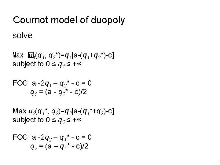
Cournot model of duopoly solve Max � u 1(q 1, q 2*)=q 1[a-(q 1+q 2*)-c] subject to 0 ≤ q 1 ≤ +∞ FOC: a -2 q 1 – q 2* - c = 0 q 1 = (a - q 2* - c)/2 Max u 2(q 1*, q 2)=q 2[a-(q 1*+q 2)-c] subject to 0 ≤ q 2 ≤ +∞ FOC: a -2 q 2 – q 1* - c = 0 q 2 = (a – q 1* - c)/2

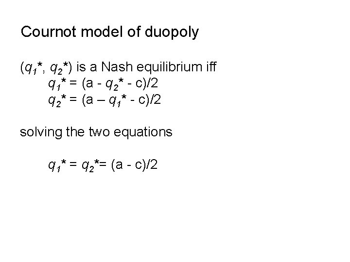
Cournot model of duopoly (q 1*, q 2*) is a Nash equilibrium iff q 1* = (a - q 2* - c)/2 q 2* = (a – q 1* - c)/2 solving the two equations q 1* = q 2*= (a - c)/2

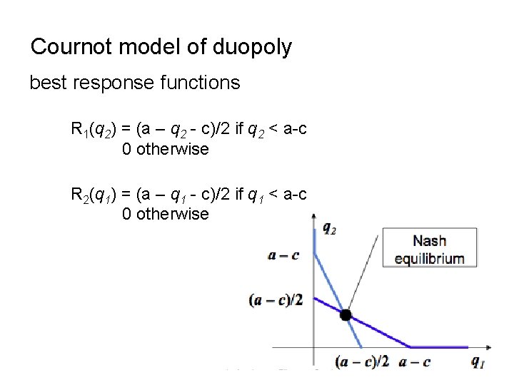
Cournot model of duopoly best response functions R 1(q 2) = (a – q 2 - c)/2 if q 2 < a-c 0 otherwise R 2(q 1) = (a – q 1 - c)/2 if q 1 < a-c 0 otherwise

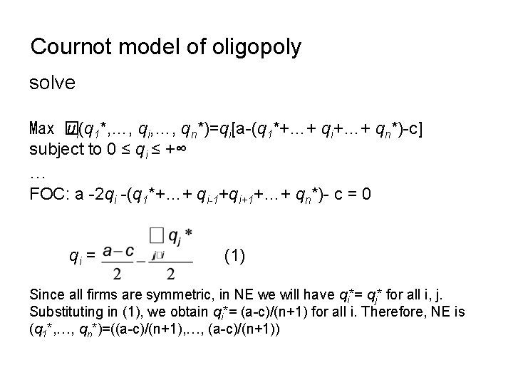
Cournot model of oligopoly solve Max � ui(q 1*, …, qi, …, qn*)=qi[a-(q 1*+…+ qi+…+ qn*)-c] subject to 0 ≤ qi ≤ +∞ … FOC: a -2 qi -(q 1*+…+ qi-1+qi+1+…+ qn*)- c = 0 qi = (1) Since all firms are symmetric, in NE we will have qi*= qj* for all i, j. Substituting in (1), we obtain qi*= (a-c)/(n+1) for all i. Therefore, NE is (q 1*, …, qn*)=((a-c)/(n+1), …, (a-c)/(n+1))

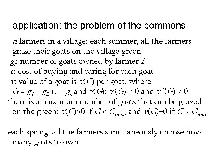
application: the problem of the commons n farmers in a village; each summer, all the farmers graze their goats on the village green gi: number of goats owned by farmer I c: cost of buying and caring for each goat v: value of a goat is v(G) per goat, where G = g 1 + g 2 +. . . +gn and v(G): v’(G) < 0 and v’’(G) < 0 there is a maximum number of goats that can be grazed on the green: v(G)>0 if G < Gmax, and v(G)=0 if G ≥ Gmax each spring, all the farmers simultaneously choose how many goats to own

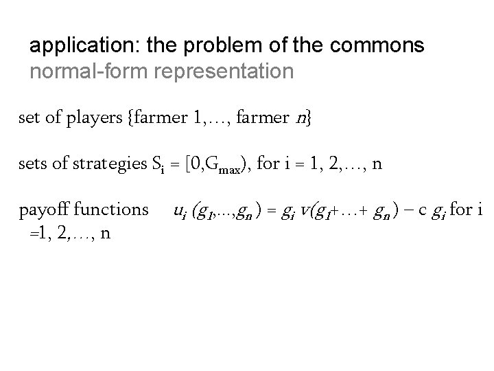
application: the problem of the commons normal-form representation set of players {farmer 1, …, farmer n} sets of strategies Si = [0, Gmax), for i = 1, 2, …, n payoff functions =1, 2, …, n ui (g 1, . . . , gn ) = gi v(g 1+…+ gn ) – c gi for i

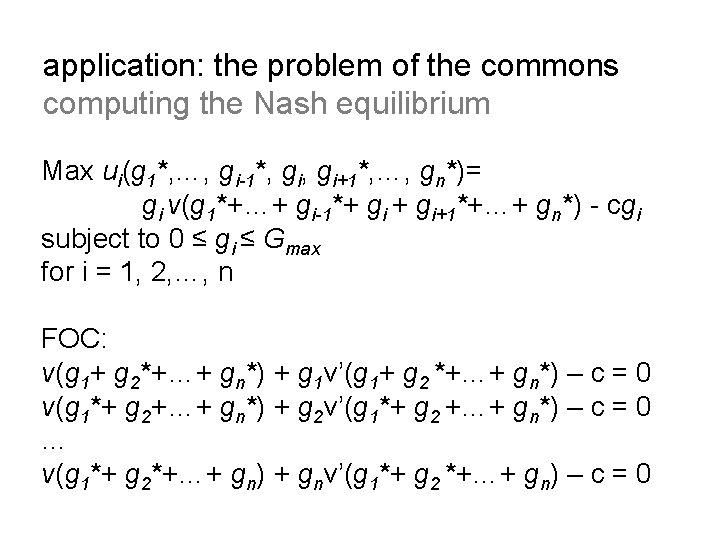
application: the problem of the commons computing the Nash equilibrium Max ui(g 1*, …, gi-1*, gi+1*, …, gn*)= gi v(g 1*+…+ gi-1*+ gi+1*+…+ gn*) - cgi subject to 0 ≤ gi ≤ Gmax for i = 1, 2, …, n FOC: v(g 1+ g 2*+…+ gn*) + g 1 v’(g 1+ g 2 *+…+ gn*) – c = 0 v(g 1*+ g 2+…+ gn*) + g 2 v’(g 1*+ g 2 +…+ gn*) – c = 0 … v(g 1*+ g 2*+…+ gn) + gnv’(g 1*+ g 2 *+…+ gn) – c = 0

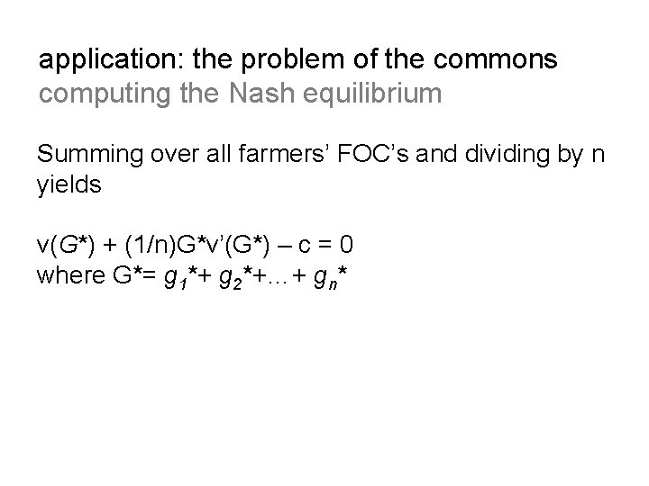
application: the problem of the commons computing the Nash equilibrium Summing over all farmers’ FOC’s and dividing by n yields v(G*) + (1/n)G*v’(G*) – c = 0 where G*= g 1*+ g 2*+…+ gn*

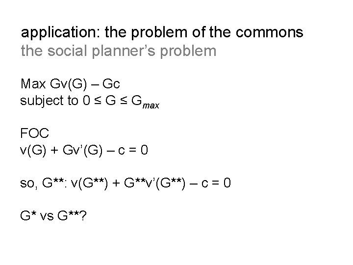
application: the problem of the commons the social planner’s problem Max Gv(G) – Gc subject to 0 ≤ Gmax FOC v(G) + Gv’(G) – c = 0 so, G**: v(G**) + G**v’(G**) – c = 0 G* vs G**?

to solve: all exercises except for ex. 3 and 7