Nonstationary GEV Models Hidden Markov Models An Introduction

Nonstationary GEV Models Hidden Markov Models An Introduction to Statistical Modeling of Extreme Values Stuart Coles Hidden Markov Models for Time Series Walter Zucchini Coles (2001), Zucchini (2016)

Outline I. Nonstationary GEV models ‐ Stationary GEV modeling ‐ Nonstationary GEV modeling ‐ R code demonstration II. Hidden Markov models ‐ Mixture models ‐ Markov chains ‐ HMMs ‐ R code demonstration

Outline I. Nonstationary GEV models ‐ Stationary GEV modeling ‐ Nonstationary GEV modeling ‐ R code demonstration II. Hidden Markov models ‐ Mixture models ‐ Markov chains ‐ HMMs ‐ R code demonstration

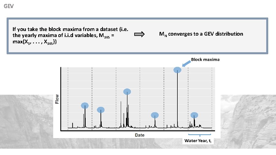
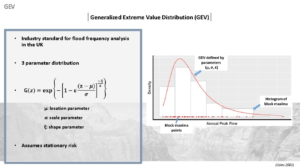
GEV If you take the block maxima from a dataset (i. e. the yearly maxima of i. i. d variables, M 365 = max{X 1, . . . , X 365}) MN converges to a GEV distribution

GEV Generalized Extreme Value Distribution (GEV) • Industry standard for flood frequency analysis in the UK • 3 parameter distribution • µ: location parameter σ: scale parameter ξ: shape parameter • Assumes stationary risk (Coles 2001)

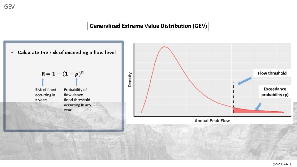
GEV Generalized Extreme Value Distribution (GEV) • Calculate the risk of exceeding a flow level (Coles 2001)

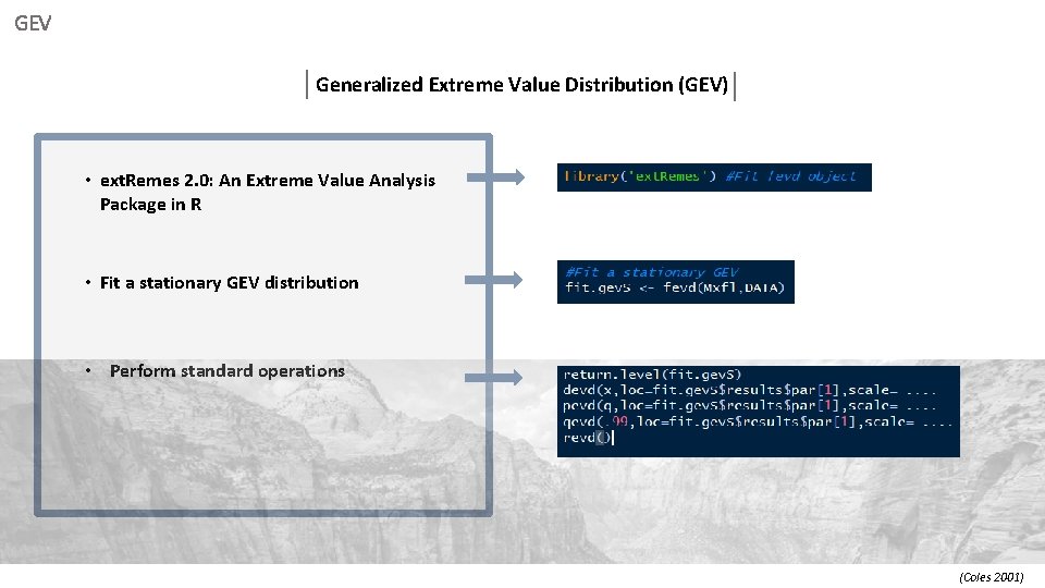
GEV Generalized Extreme Value Distribution (GEV) • ext. Remes 2. 0: An Extreme Value Analysis Package in R • Fit a stationary GEV distribution • Perform standard operations (Coles 2001)

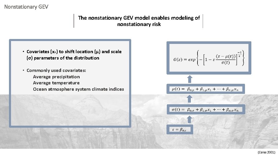
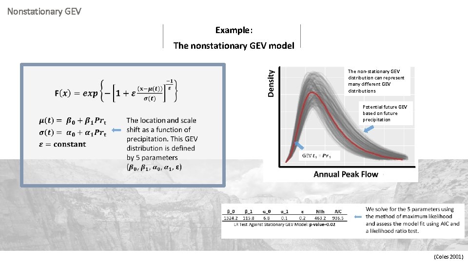
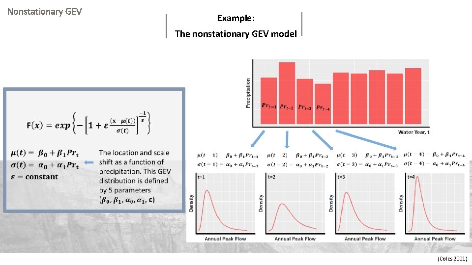
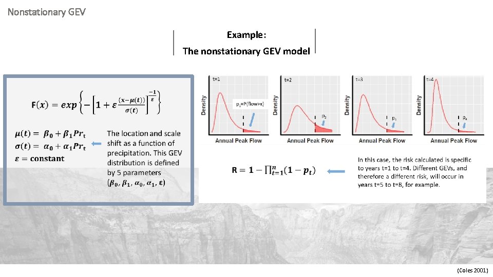
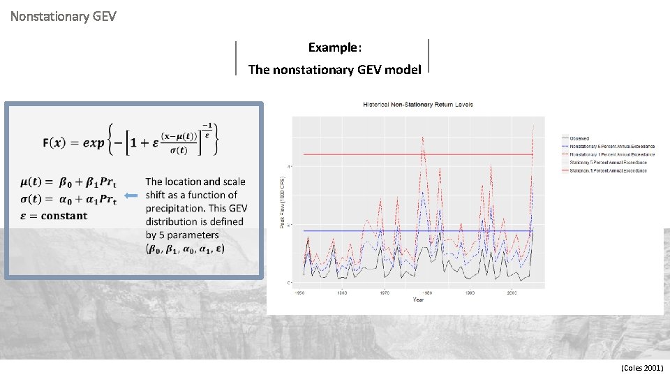
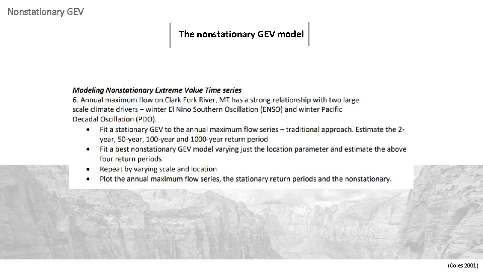
Nonstationary GEV The nonstationary GEV model enables modeling of nonstationary risk • Covariates (xn) to shift location (µ) and scale (σ) parameters of the distribution • Commonly used covariates: Average precipitation Average temperature Ocean atmosphere system climate indices (Coles 2001)

Nonstationary GEV Example: The nonstationary GEV model The non‐stationary GEV distribution can represent many different GEV distributions Potential future GEV based on future precipitation (Coles 2001)

Nonstationary GEV Example: The nonstationary GEV model (Coles 2001)

Nonstationary GEV Example: The nonstationary GEV model (Coles 2001)

Nonstationary GEV Example: The nonstationary GEV model (Coles 2001)

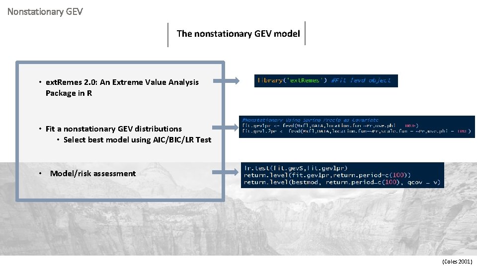
Nonstationary GEV The nonstationary GEV model • ext. Remes 2. 0: An Extreme Value Analysis Package in R • Fit a nonstationary GEV distributions • Select best model using AIC/BIC/LR Test • Model/risk assessment (Coles 2001)

Nonstationary GEV The nonstationary GEV model (Coles 2001)

Outline I. Nonstationary GEV models ‐ Stationary GEV modeling ‐ Nonstationary GEV modeling ‐ R code demonstration II. Hidden Markov models ‐ Mixture models ‐ Markov chains ‐ HMMs ‐ R code demonstration

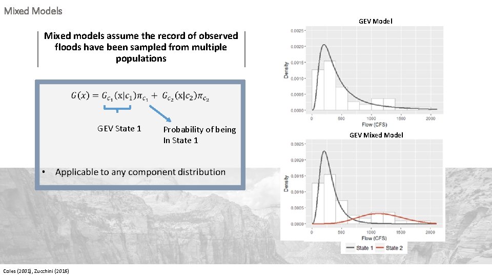
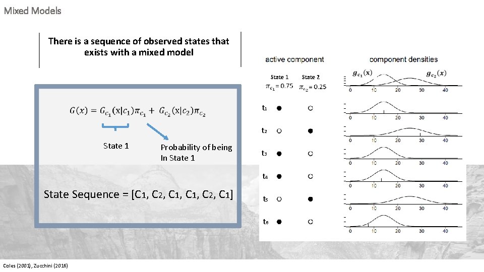
Mixed Models GEV Model Mixed models assume the record of observed floods have been sampled from multiple populations GEV State 1 Coles (2001), Zucchini (2016) Probability of being In State 1 GEV Mixed Model

Mixed Models There is a sequence of observed states that exists with a mixed model State 1 t 1 t 2 State 1 Probability of being In State 1 t 3 t 4 State Sequence = [C 1, C 2, C 1] t 5 t 6 Coles (2001), Zucchini (2016) State 2

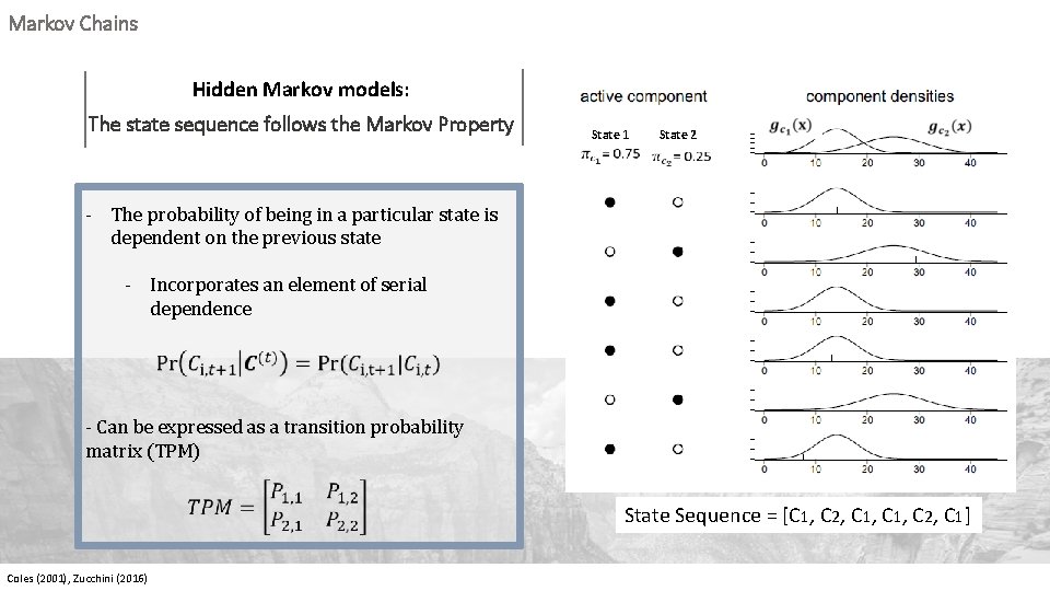
Markov Chains Hidden Markov models: The state sequence follows the Markov Property State 1 State 2 - The probability of being in a particular state is dependent on the previous state - Incorporates an element of serial dependence - Can be expressed as a transition probability matrix (TPM) State Sequence = [C 1, C 2, C 1] Coles (2001), Zucchini (2016)

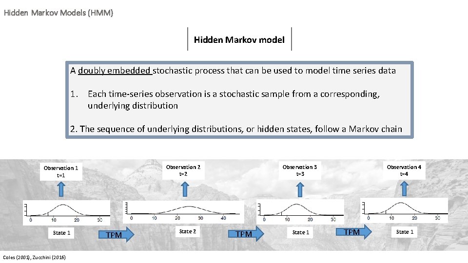
Hidden Markov Models (HMM) Hidden Markov model A doubly embedded stochastic process that can be used to model time series data 1. Each time‐series observation is a stochastic sample from a corresponding, underlying distribution 2. The sequence of underlying distributions, or hidden states, follow a Markov chain State 1 Coles (2001), Zucchini (2016) TPM State 2 Observation 4 t=4 Observation 3 t=3 Observation 2 t=2 Observation 1 t=1 TPM State 1

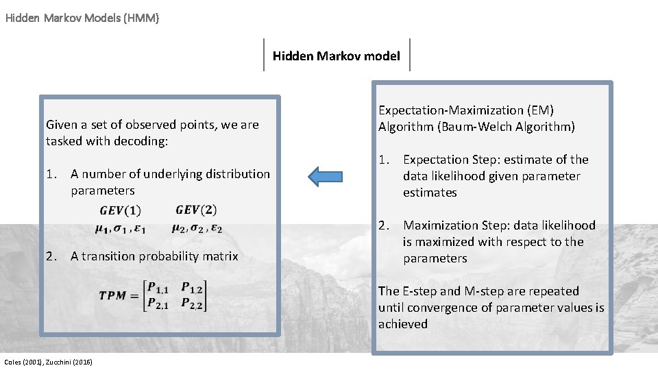
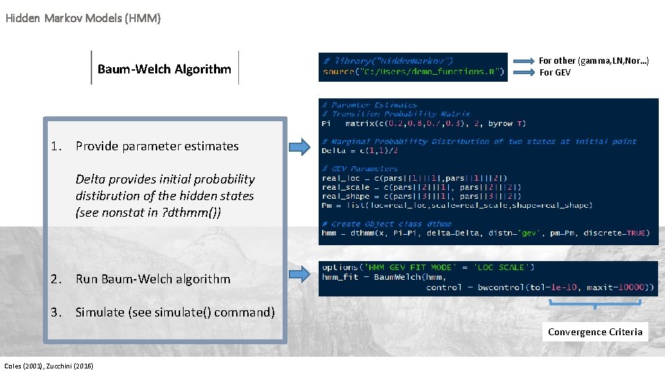
Hidden Markov Models (HMM) Hidden Markov model Given a set of observed points, we are tasked with decoding: 1. A number of underlying distribution parameters 2. A transition probability matrix Coles (2001), Zucchini (2016) Expectation‐Maximization (EM) Algorithm (Baum‐Welch Algorithm) 1. Expectation Step: estimate of the data likelihood given parameter estimates 2. Maximization Step: data likelihood is maximized with respect to the parameters The E‐step and M‐step are repeated until convergence of parameter values is achieved

Hidden Markov Models (HMM) Baum-Welch Algorithm For other (gamma, LN, Nor…) For GEV 1. Provide parameter estimates Delta provides initial probability distibrution of the hidden states (see nonstat in ? dthmm()) 2. Run Baum‐Welch algorithm 3. Simulate (see simulate() command) Convergence Criteria Coles (2001), Zucchini (2016)

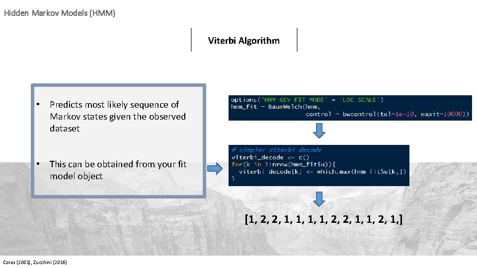
Hidden Markov Models (HMM) Viterbi Algorithm • Predicts most likely sequence of Markov states given the observed dataset • This can be obtained from your fit model object [1, 2, 2, 1, 1, 2, 1, ] Coles (2001), Zucchini (2016)

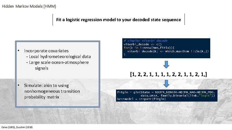
Hidden Markov Models (HMM) Fit a logistic regression model to your decoded state sequence • Incorporate covariates ‐ Local hydrometeorological data ‐ Large scale ocean‐atmosphere signals • Simulate: akin to using nonhomogeneous transition probability matrix Coles (2001), Zucchini (2016) [1, 2, 2, 1, 1, 2, 1, ]

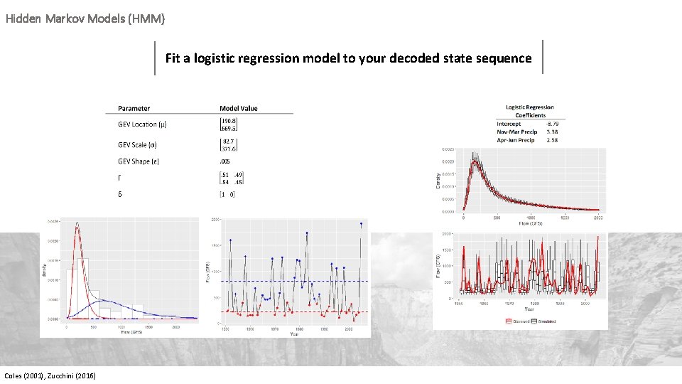
Hidden Markov Models (HMM) Fit a logistic regression model to your decoded state sequence Coles (2001), Zucchini (2016)

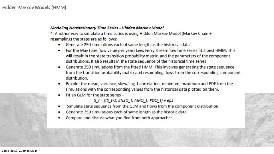
Hidden Markov Models (HMM) Coles (2001), Zucchini (2016)