NonStandard Databases and Data Mining Dynamic Bayesian Networks
Non-Standard Databases and Data Mining Dynamic Bayesian Networks Prof. Dr. Ralf Möller Universität zu Lübeck Institut für Informationssystem
Time and Uncertainty • • • The world changes, we need to track and predict it Examples: diabetes management, traffic monitoring Uncertainty is everywhere Need temporal probabilistic graphical models Basic idea: copy state and evidence variables for each time step • Xt – set of unobservable state variables at time t – e. g. , Blood. Sugart, Stomach. Contentst • Et – set of evidence variables at time t – e. g. , Measured. Blood. Sugart, Pulse. Ratet, Food. Eatent • Assumes discrete time steps 2
States and Observations • Process of change viewed as series of snapshots, each describing the state of the world at a particular time Time slice involves a set of random variables indexed by t: • – – • • the set of unobservable state variables Xt the set of observable evidence variable Et The observation at time t is Et = et for some set of values et The notation Xa: b denotes the set of variables from Xa to Xb 3

Dynamic Bayesian Networks • How can we model dynamic situations with a Bayesian network? • Example: Is it raining today? next step: specify dependencies among the variables. The term “dynamic” means we are modeling a dynamic system, not that the network structure changes over time. 4
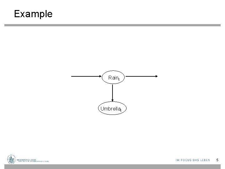
Example Raint Umbrellat 5
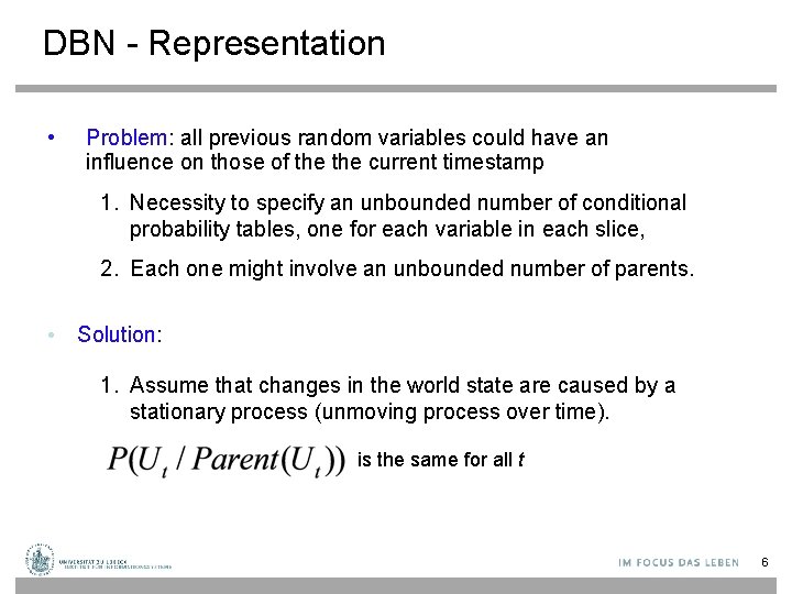
DBN - Representation • Problem: all previous random variables could have an influence on those of the current timestamp 1. Necessity to specify an unbounded number of conditional probability tables, one for each variable in each slice, 2. Each one might involve an unbounded number of parents. • Solution: 1. Assume that changes in the world state are caused by a stationary process (unmoving process over time). is the same for all t 6
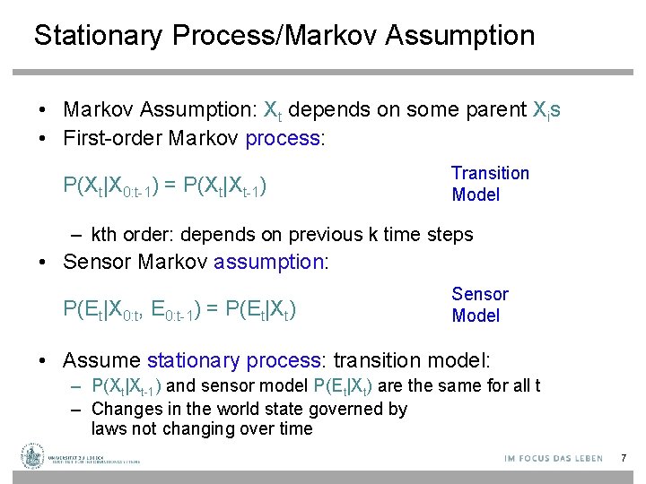
Stationary Process/Markov Assumption • Markov Assumption: Xt depends on some parent Xis • First-order Markov process: P(Xt|X 0: t-1) = P(Xt|Xt-1) Transition Model – kth order: depends on previous k time steps • Sensor Markov assumption: P(Et|X 0: t, E 0: t-1) = P(Et|Xt) Sensor Model • Assume stationary process: transition model: – P(Xt|Xt-1) and sensor model P(Et|Xt) are the same for all t – Changes in the world state governed by laws not changing over time 7
Dynamic Bayesian Networks • There are two possible fixes if the approximation is too inaccurate: – Increasing the order of the Markov process model. For example, adding as a parent of , which might give slightly more accurate predictions. – Increasing the set of state variables. For example, adding to allow to incorporate historical records of rainy seasons, or adding , and Pressure to allow to use a physical model of rainy conditions. 8
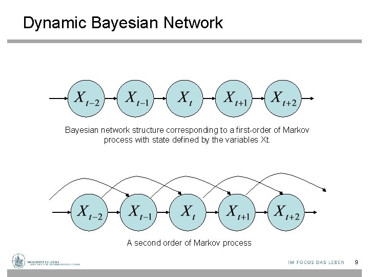
Dynamic Bayesian Network Bayesian network structure corresponding to a first-order of Markov process with state defined by the variables Xt. A second order of Markov process 9
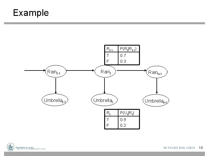
Example Raint-1 Umbrellat-1 Rt-1 P(Rt|Rt-1) T F 0. 7 0. 3 Raint+1 Umbrellat+1 Rt P(Ut|Rt) T F 0. 9 0. 2 10
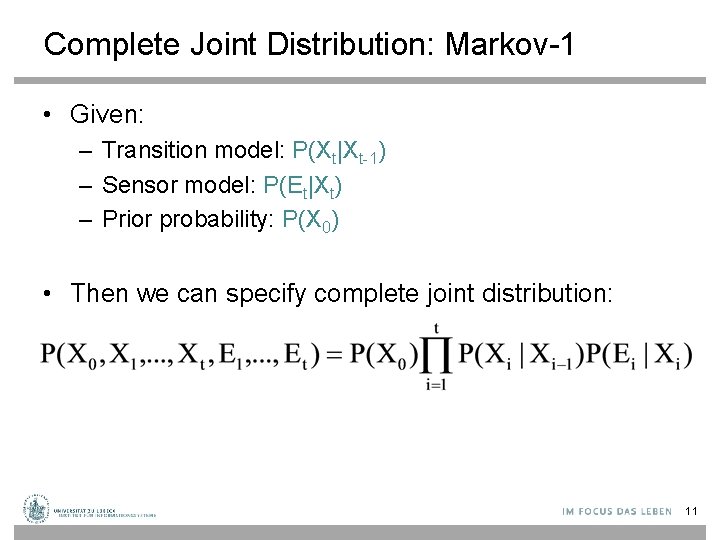
Complete Joint Distribution: Markov-1 • Given: – Transition model: P(Xt|Xt-1) – Sensor model: P(Et|Xt) – Prior probability: P(X 0) • Then we can specify complete joint distribution: 11
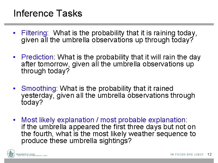
Inference Tasks • Filtering: What is the probability that it is raining today, given all the umbrella observations up through today? • Prediction: What is the probability that it will rain the day after tomorrow, given all the umbrella observations up through today? • Smoothing: What is the probability that it rained yesterday, given all the umbrella observations through today? • Most likely explanation / most probable explanation: if the umbrella appeared the first three days but not on the fourth, what is the most likely weather sequence to produce these umbrella sightings? 12
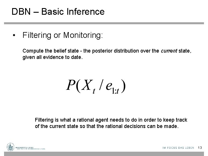
DBN – Basic Inference • Filtering or Monitoring: Compute the belief state - the posterior distribution over the current state, given all evidence to date. Filtering is what a rational agent needs to do in order to keep track of the current state so that the rational decisions can be made. 13

DBN – Basic Inference • Filtering cont. Given the results of filtering up to time t, one can easily compute the result for t+1 from the new evidence (for some function f) (dividing up the evidence) (using Bayes’ Theorem) (by the Markov property of evidence) α is a normalizing constant used to make probabilities sum up to 1. 14
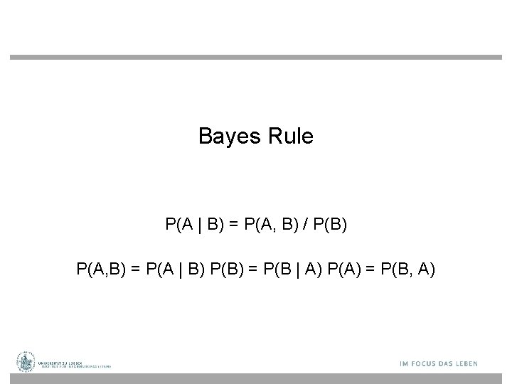
Bayes Rule P(A | B) = P(A, B) / P(B) P(A, B) = P(A | B) P(B) = P(B | A) P(A) = P(B, A)
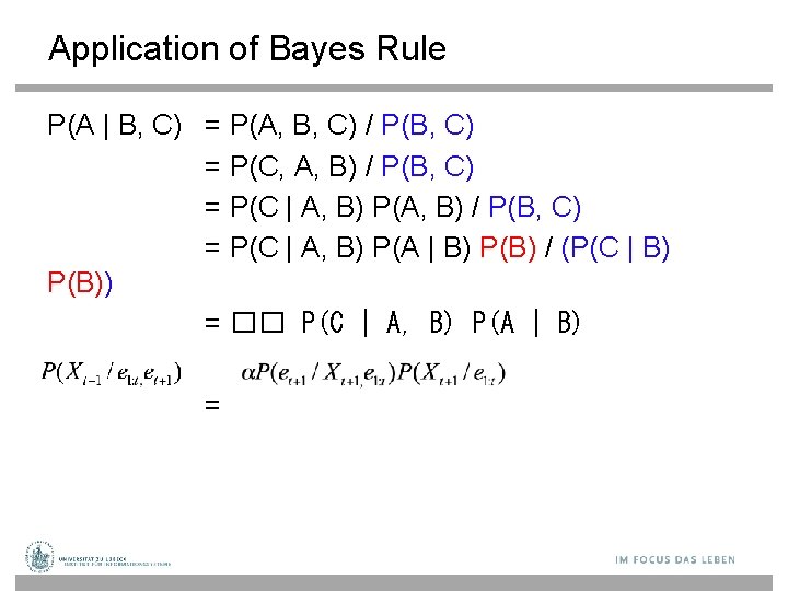
Application of Bayes Rule P(A | B, C) = P(A, B, C) / P(B, C) = P(C, A, B) / P(B, C) = P(C | A, B) P(A | B) P(B) / (P(C | B) P(B)) = �� P(C | A, B) P(A | B) =
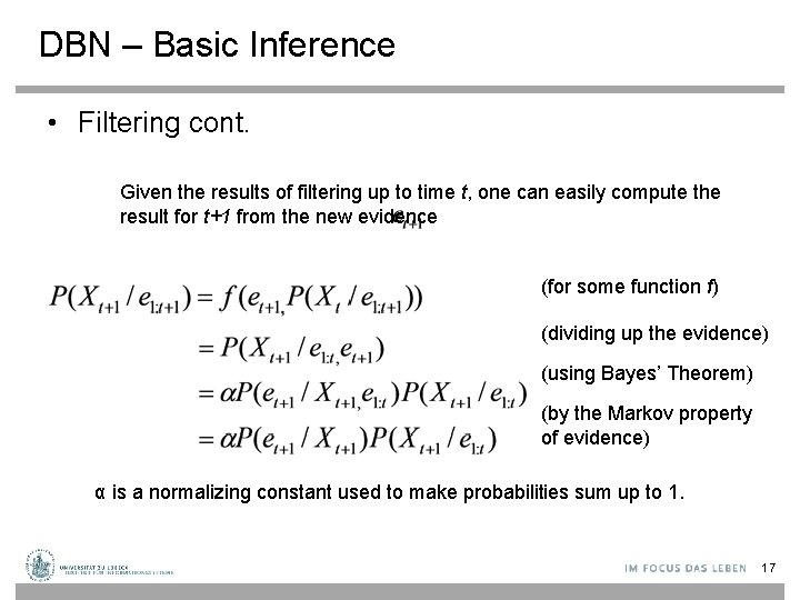
DBN – Basic Inference • Filtering cont. Given the results of filtering up to time t, one can easily compute the result for t+1 from the new evidence (for some function f) (dividing up the evidence) (using Bayes’ Theorem) (by the Markov property of evidence) α is a normalizing constant used to make probabilities sum up to 1. 17
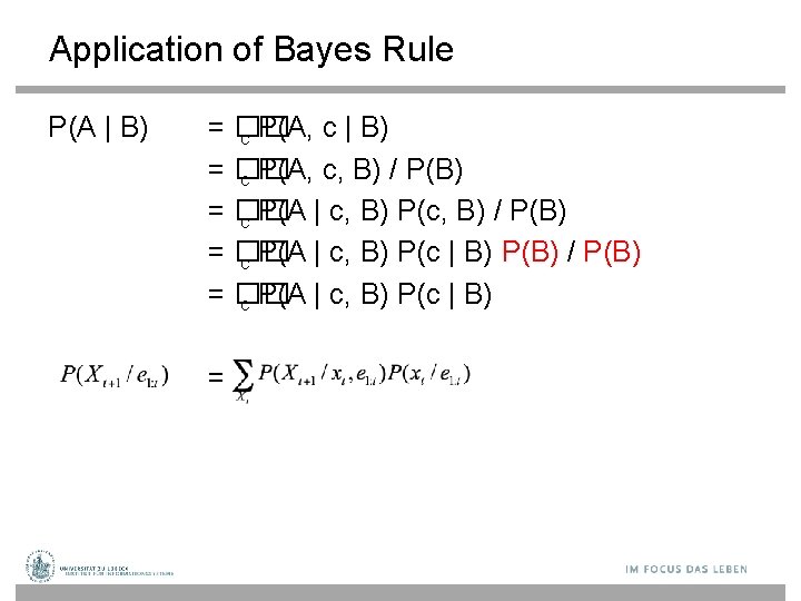
Application of Bayes Rule P(A | B) = �� c P(A, c, B) / P(B) = �� c P(A | c, B) P(c | B) P(B) / P(B) = �� c P(A | c, B) P(c | B) =

DBN – Basic Inference • Filtering cont. The second term represents a one-step prediction of the next step, and the first term updates this with the new evidence. Now we obtain the one-step prediction for the next step by conditioning on the current state Xt: (using the Markov property) 19
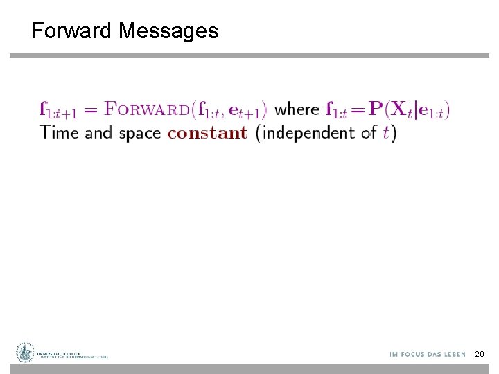
Forward Messages 20
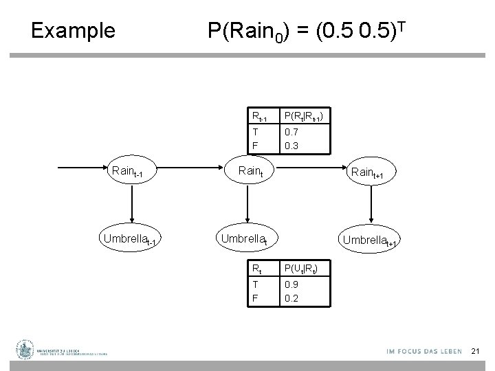
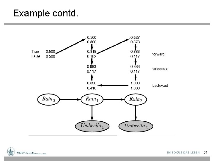
Example Raint-1 Umbrellat-1 P(Rain 0) = (0. 5)T Rt-1 P(Rt|Rt-1) T F 0. 7 0. 3 Raint+1 Umbrellat+1 Rt P(Ut|Rt) T F 0. 9 0. 2 21
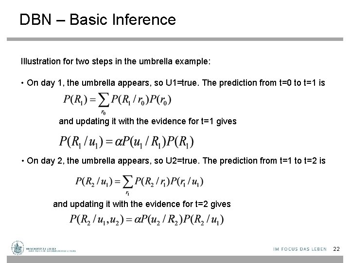
DBN – Basic Inference Illustration for two steps in the umbrella example: • On day 1, the umbrella appears, so U 1=true. The prediction from t=0 to t=1 is and updating it with the evidence for t=1 gives • On day 2, the umbrella appears, so U 2=true. The prediction from t=1 to t=2 is and updating it with the evidence for t=2 gives 22
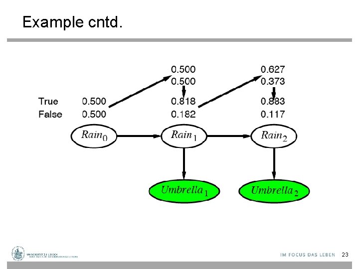
Example cntd. 23
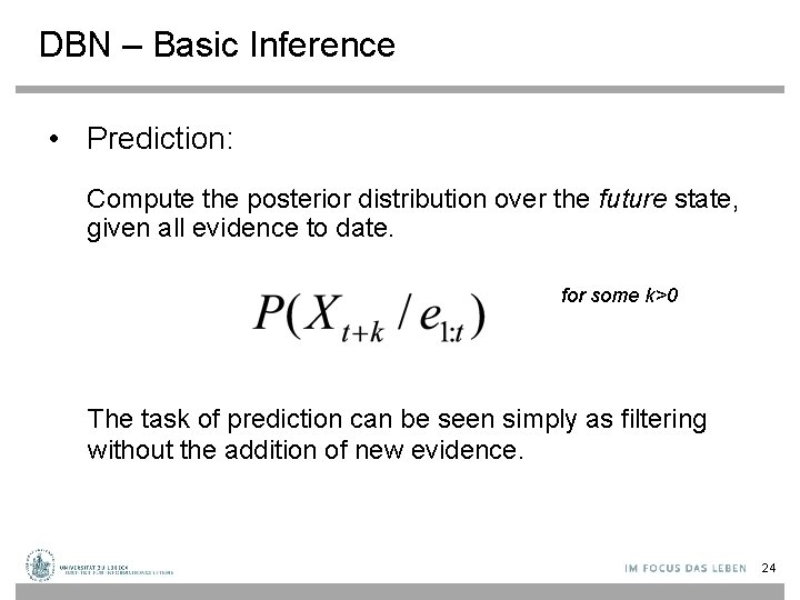
DBN – Basic Inference • Prediction: Compute the posterior distribution over the future state, given all evidence to date. for some k>0 The task of prediction can be seen simply as filtering without the addition of new evidence. 24
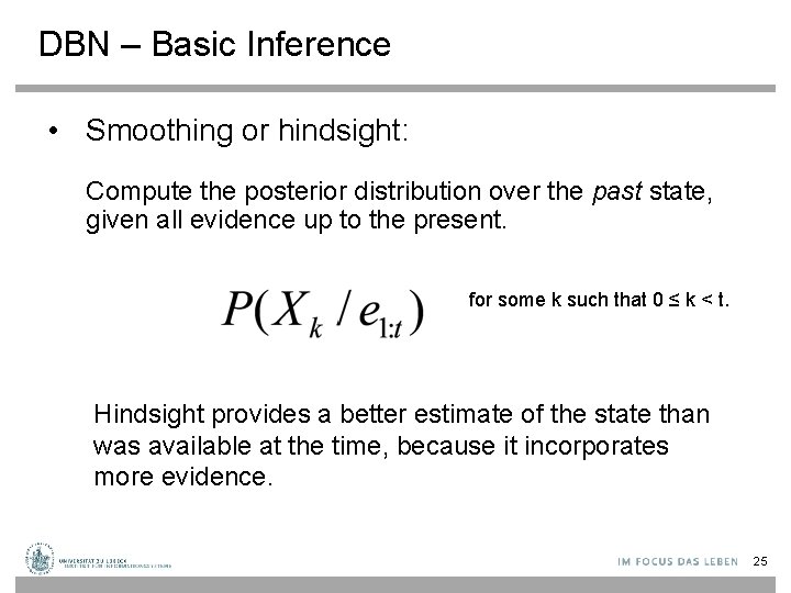
DBN – Basic Inference • Smoothing or hindsight: Compute the posterior distribution over the past state, given all evidence up to the present. for some k such that 0 ≤ k < t. Hindsight provides a better estimate of the state than was available at the time, because it incorporates more evidence. 25

Smoothing 26
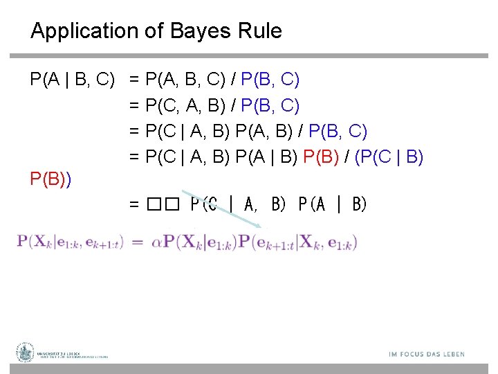
Application of Bayes Rule P(A | B, C) = P(A, B, C) / P(B, C) = P(C, A, B) / P(B, C) = P(C | A, B) P(A | B) P(B) / (P(C | B) P(B)) = �� P(C | A, B) P(A | B)
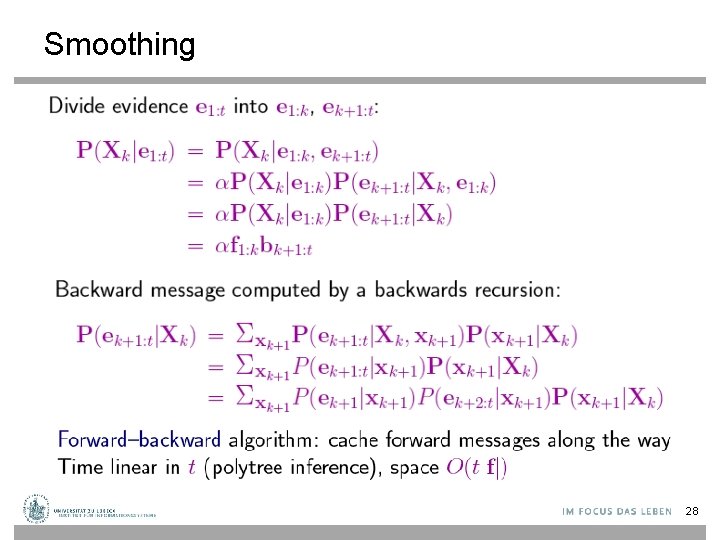
Smoothing 28
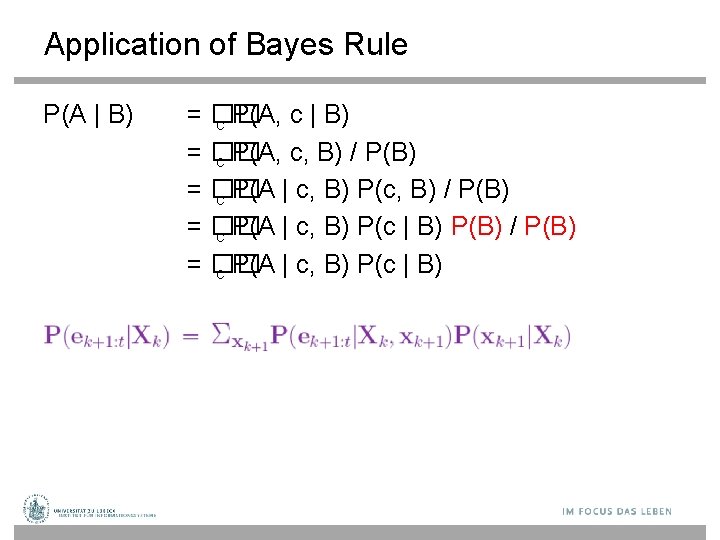
Application of Bayes Rule P(A | B) = �� c P(A, c, B) / P(B) = �� c P(A | c, B) P(c | B) P(B) / P(B) = �� c P(A | c, B) P(c | B)

Smoothing 30
Example contd. 31
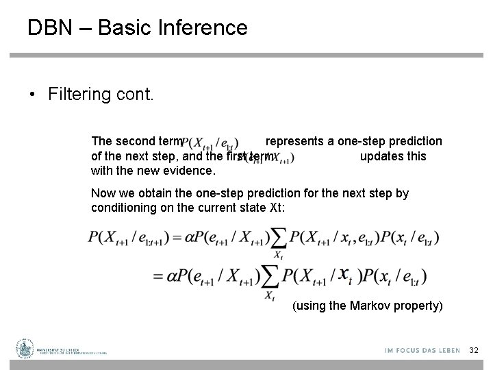
DBN – Basic Inference • Filtering cont. The second term represents a one-step prediction of the next step, and the first term updates this with the new evidence. Now we obtain the one-step prediction for the next step by conditioning on the current state Xt: (using the Markov property) 32
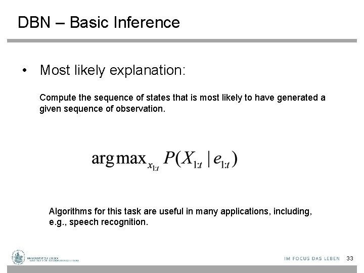
DBN – Basic Inference • Most likely explanation: Compute the sequence of states that is most likely to have generated a given sequence of observation. Algorithms for this task are useful in many applications, including, e. g. , speech recognition. 33
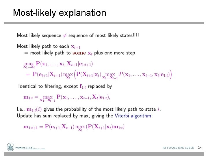
Most-likely explanation 34
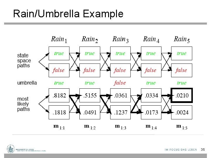
Rain/Umbrella Example 35
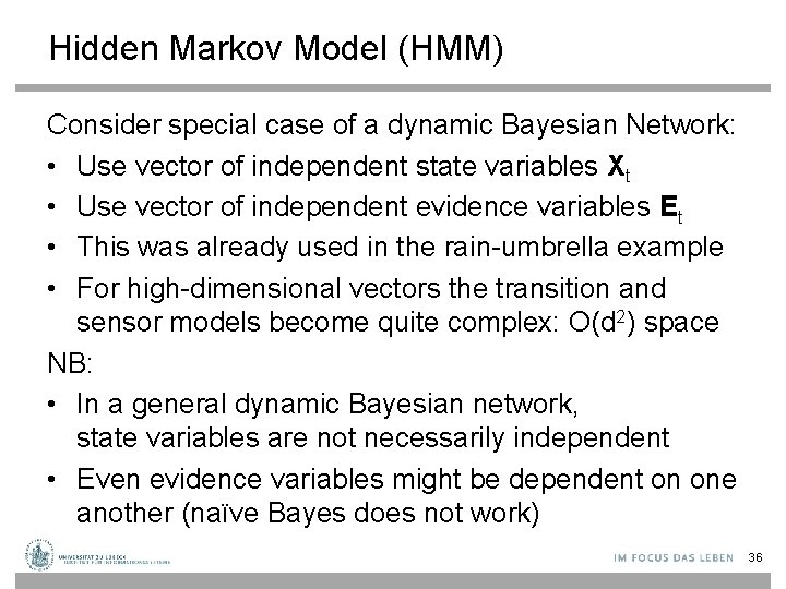
Hidden Markov Model (HMM) Consider special case of a dynamic Bayesian Network: • Use vector of independent state variables Xt • Use vector of independent evidence variables Et • This was already used in the rain-umbrella example • For high-dimensional vectors the transition and sensor models become quite complex: O(d 2) space NB: • In a general dynamic Bayesian network, state variables are not necessarily independent • Even evidence variables might be dependent on one another (naïve Bayes does not work) 36
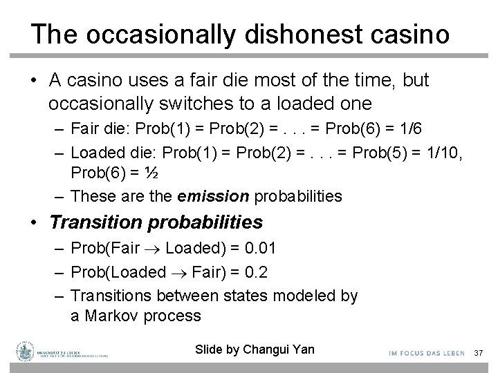
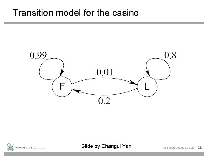
The occasionally dishonest casino • A casino uses a fair die most of the time, but occasionally switches to a loaded one – Fair die: Prob(1) = Prob(2) =. . . = Prob(6) = 1/6 – Loaded die: Prob(1) = Prob(2) =. . . = Prob(5) = 1/10, Prob(6) = ½ – These are the emission probabilities • Transition probabilities – Prob(Fair Loaded) = 0. 01 – Prob(Loaded Fair) = 0. 2 – Transitions between states modeled by a Markov process Slide by Changui Yan 37
Transition model for the casino Slide by Changui Yan 38
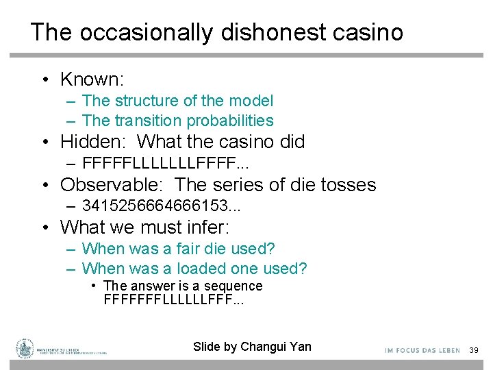
The occasionally dishonest casino • Known: – The structure of the model – The transition probabilities • Hidden: What the casino did – FFFFFLLLLLLLFFFF. . . • Observable: The series of die tosses – 3415256664666153. . . • What we must infer: – When was a fair die used? – When was a loaded one used? • The answer is a sequence FFFFFFFLLLLLLFFF. . . Slide by Changui Yan 39
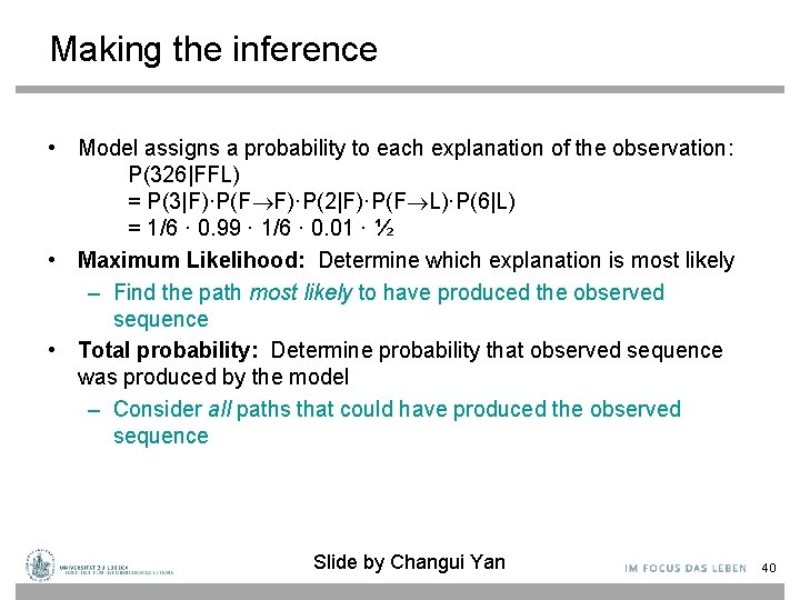
Making the inference • Model assigns a probability to each explanation of the observation: P(326|FFL) = P(3|F)·P(F F)·P(2|F)·P(F L)·P(6|L) = 1/6 · 0. 99 · 1/6 · 0. 01 · ½ • Maximum Likelihood: Determine which explanation is most likely – Find the path most likely to have produced the observed sequence • Total probability: Determine probability that observed sequence was produced by the model – Consider all paths that could have produced the observed sequence Slide by Changui Yan 40
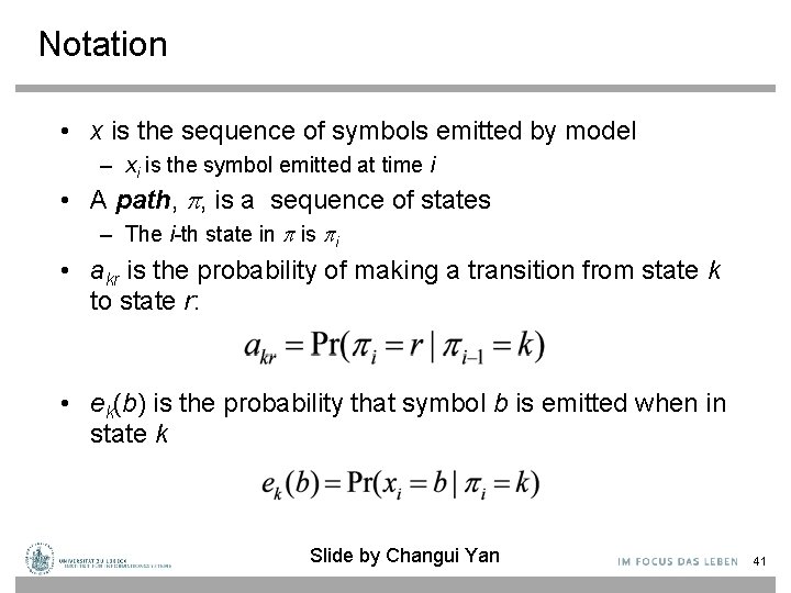
Notation • x is the sequence of symbols emitted by model – xi is the symbol emitted at time i • A path, , is a sequence of states – The i-th state in is i • akr is the probability of making a transition from state k to state r: • ek(b) is the probability that symbol b is emitted when in state k Slide by Changui Yan 41
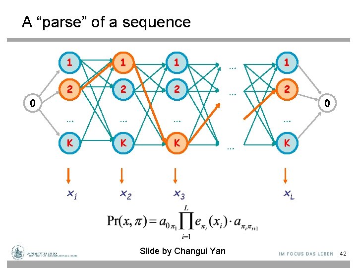
A “parse” of a sequence 0 1 1 1 … 1 2 2 2 … … … K K K x 1 x 2 x 3 Slide by Changui Yan … … 0 K x. L 42
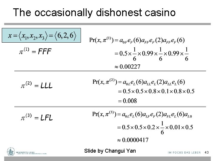
The occasionally dishonest casino Slide by Changui Yan 43
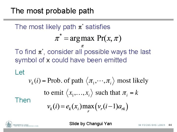
The most probable path The most likely path * satisfies To find *, consider all possible ways the last symbol of x could have been emitted Let Then Slide by Changui Yan 44
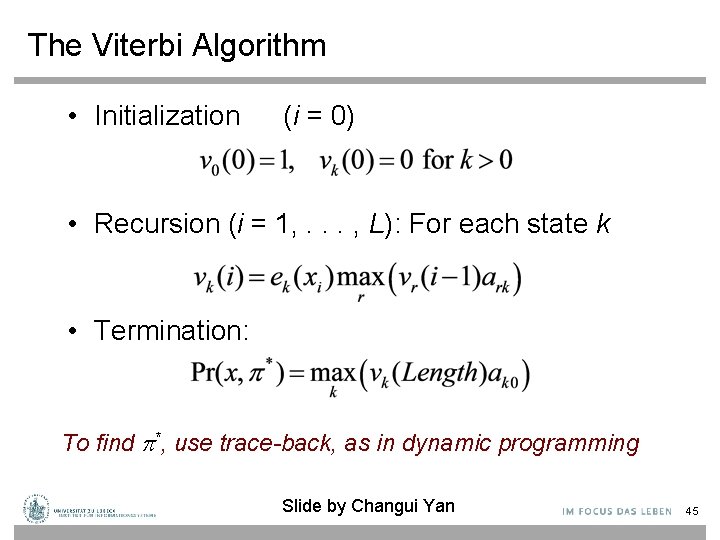
The Viterbi Algorithm • Initialization (i = 0) • Recursion (i = 1, . . . , L): For each state k • Termination: To find *, use trace-back, as in dynamic programming Slide by Changui Yan 45
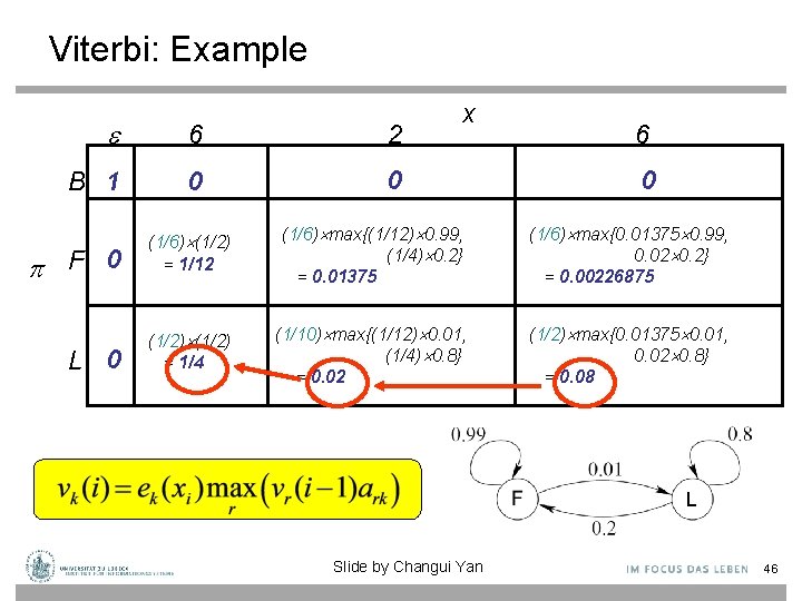
Viterbi: Example 6 2 B 1 0 0 F 0 L 0 x 6 0 (1/6) (1/2) = 1/12 (1/6) max{(1/12) 0. 99, (1/4) 0. 2} = 0. 01375 (1/6) max{0. 01375 0. 99, 0. 02 0. 2} = 0. 00226875 (1/2) = 1/4 (1/10) max{(1/12) 0. 01, (1/4) 0. 8} = 0. 02 (1/2) max{0. 01375 0. 01, 0. 02 0. 8} = 0. 08 Slide by Changui Yan 46
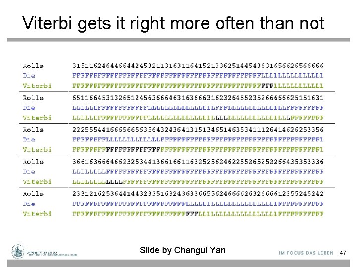
Viterbi gets it right more often than not Slide by Changui Yan 47
DBN – Special Cases • Hidden Markov Model (HMMs): Temporal probabilistic model in which the state of the process is described by a single discrete random variable. (The simplest kind of DBN ) • Kalman Filter Models (KFMs): Estimate the state of a physical system from noisy observations over time. Also known as linear dynamical systems (LDSs). 48
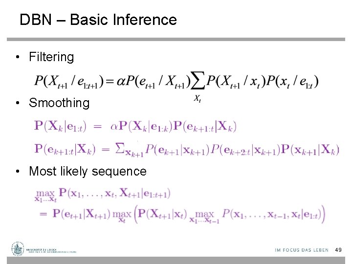
DBN – Basic Inference • Filtering • Smoothing • Most likely sequence 49
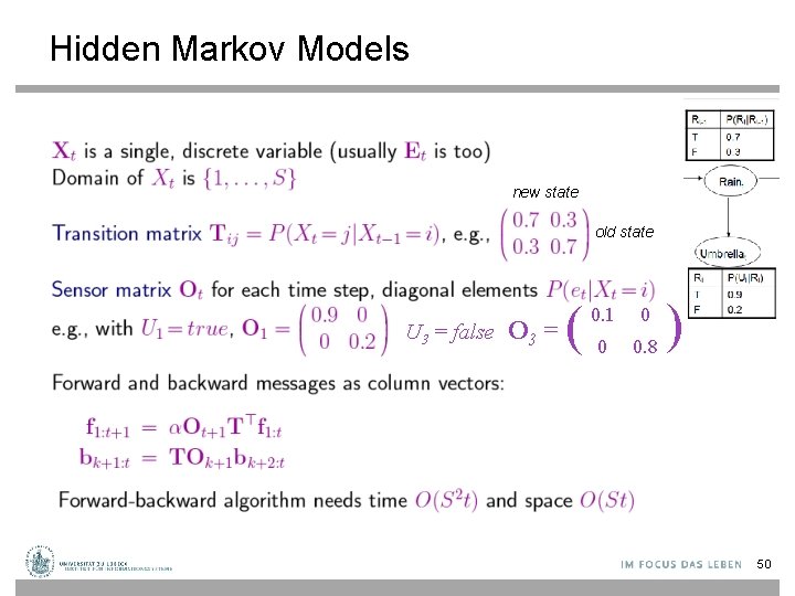
Hidden Markov Models new state old state U 3 = false O 3 = ( 0. 1 0 0 0. 8 ) 50
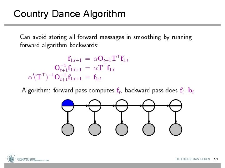
Country Dance Algorithm 51
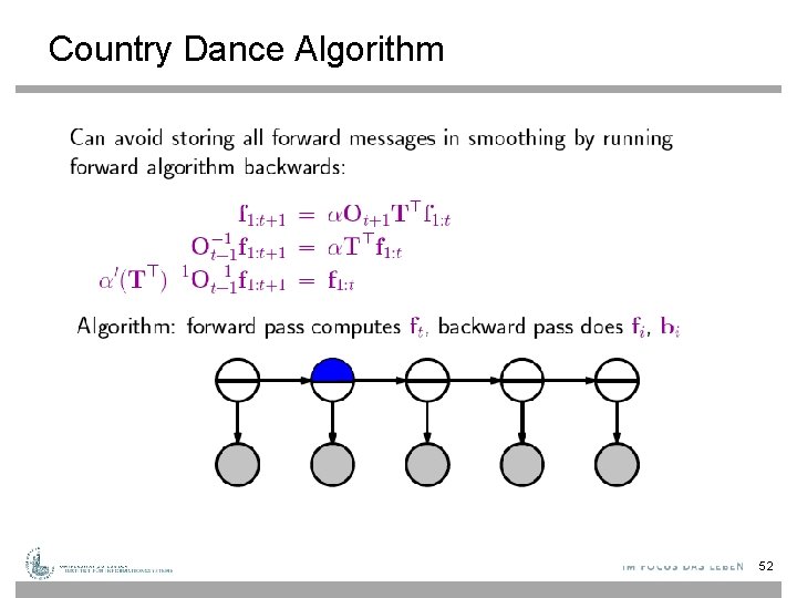
Country Dance Algorithm 52

Country Dance Algorithm 53
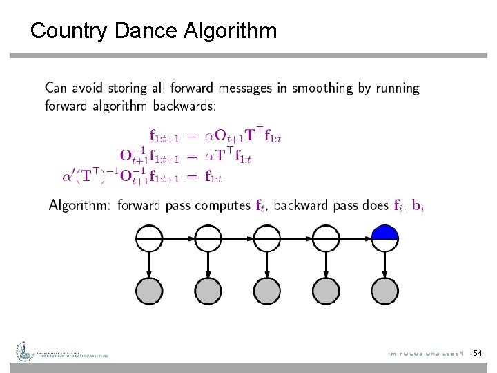
Country Dance Algorithm 54
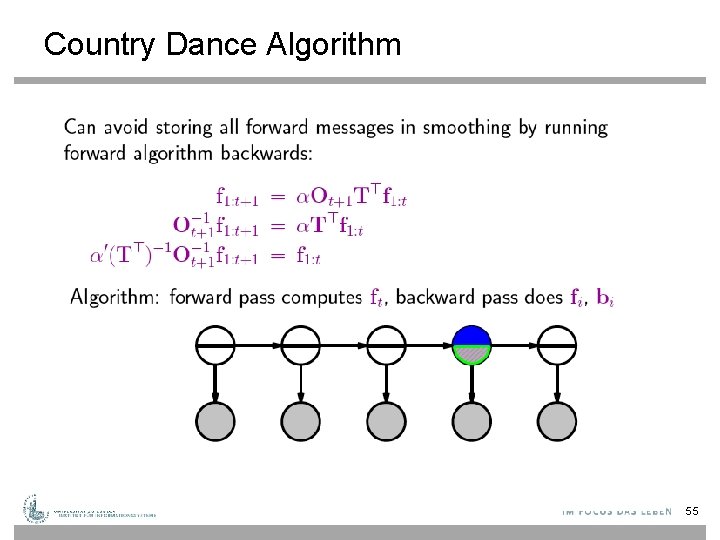
Country Dance Algorithm 55
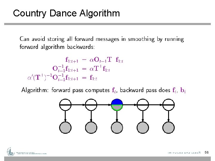
Country Dance Algorithm 56
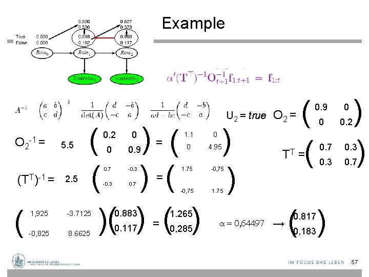
Example U 2 = true O 2 -1 = (TT)-1 = ( 5. 5 2. 5 ( ) ( ) )( ) 1, 925 -3. 7125 -0, 825 8. 6625 0. 2 0 0 0. 9 0. 7 -0. 3 0. 7 0. 883 0. 117 = = = 1. 1 0 0 4. 95 1. 75 -0, 75 1. 265 0, 285 = 0, 64497 O 2 = TT → ( ( 0. 9 0 0 0. 2 = ) ) 0. 7 0. 3 0. 7 ( ) 0. 817 0, 183 57
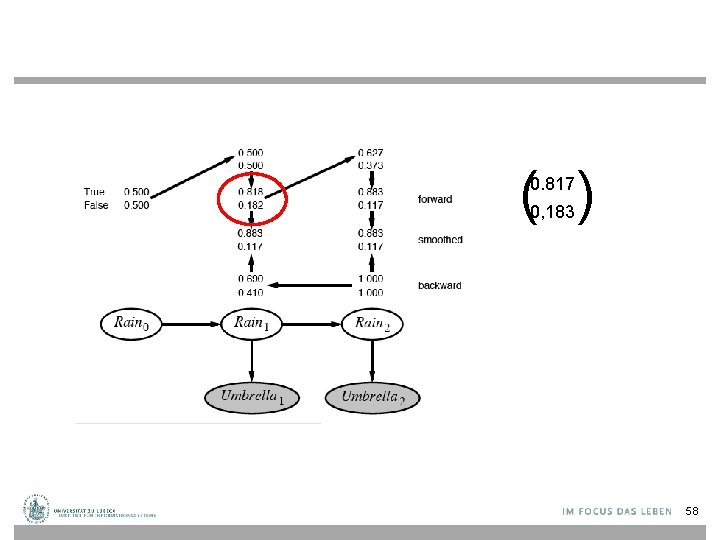
( ) 0. 817 0, 183 58
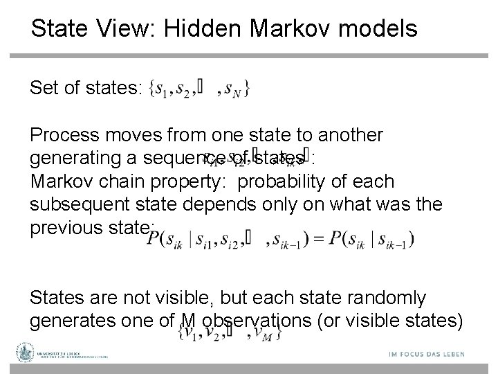
State View: Hidden Markov models Set of states: Process moves from one state to another generating a sequence of states : Markov chain property: probability of each subsequent state depends only on what was the previous state: States are not visible, but each state randomly generates one of M observations (or visible states)
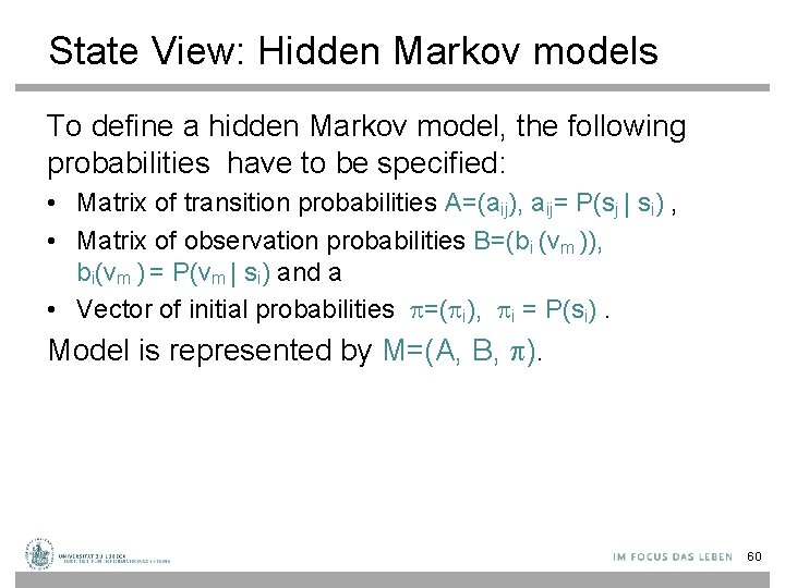
State View: Hidden Markov models To define a hidden Markov model, the following probabilities have to be specified: • Matrix of transition probabilities A=(aij), aij= P(sj | si) , • Matrix of observation probabilities B=(bi (vm )), bi(vm ) = P(vm | si) and a • Vector of initial probabilities =( i), i = P(si). Model is represented by M=(A, B, ). 60
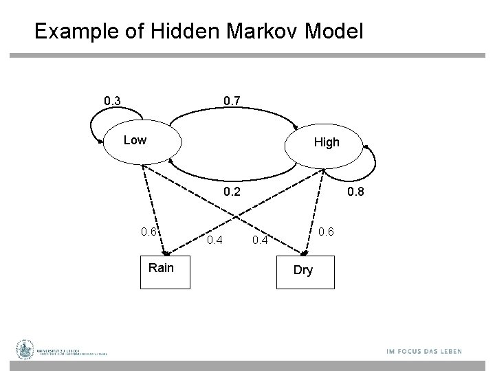
Example of Hidden Markov Model 0. 3 0. 7 Low High 0. 2 0. 6 Rain 0. 4 0. 8 0. 6 0. 4 Dry
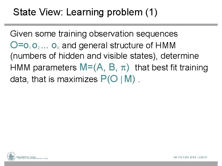
State View: Learning problem (1) Given some training observation sequences O=o 1 o 2. . . o. K and general structure of HMM (numbers of hidden and visible states), determine HMM parameters M=(A, B, ) that best fit training data, that is maximizes P(O | M).
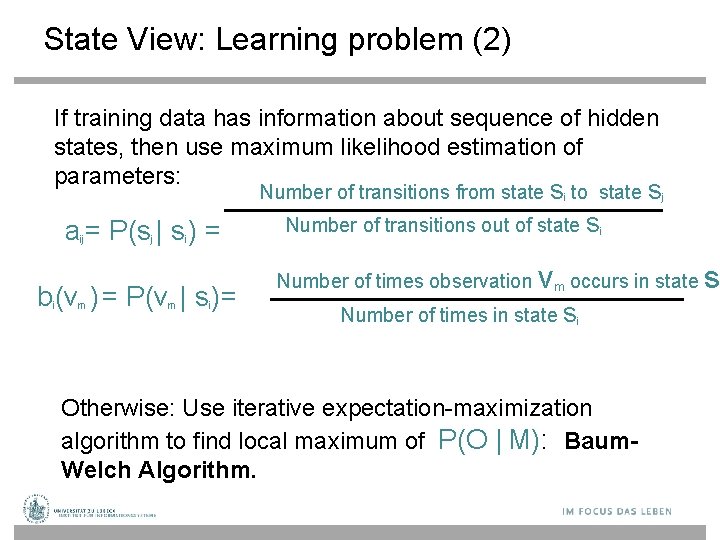
State View: Learning problem (2) If training data has information about sequence of hidden states, then use maximum likelihood estimation of parameters: Number of transitions from state si to state sj a = P(s | s ) = ij j i b (v ) = P(v | s )= i m m i Number of transitions out of state si Number of times observation v m occurs in state Number of times in state si Otherwise: Use iterative expectation-maximization algorithm to find local maximum of P(O | M): Baum. Welch Algorithm. s
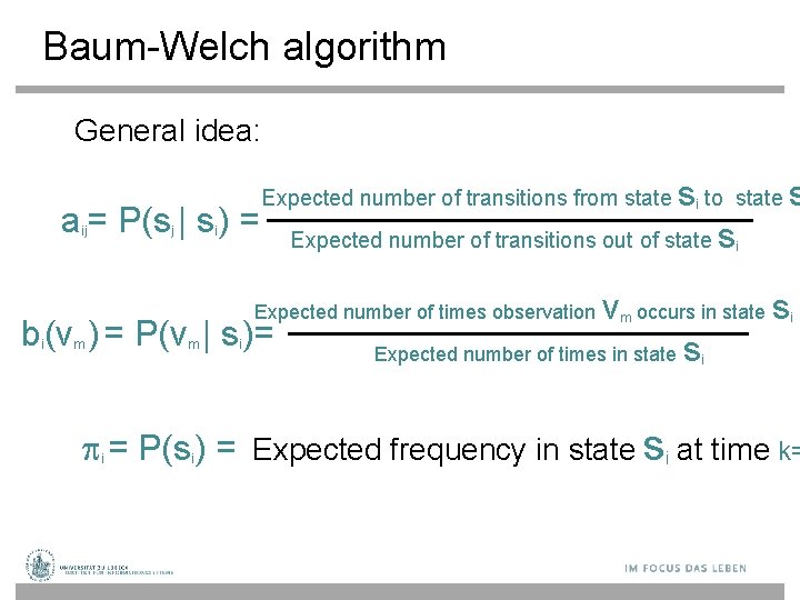
Baum-Welch algorithm General idea: s to state s a = P(s | s ) = Expected number of transitions out of state s Expected number of transitions from state ij j i i i Expected number of times observation b (v ) = P(v | s )= i m m i v m occurs in state Expected number of times in state s i = P(s ) = Expected frequency in state si at time k= i i
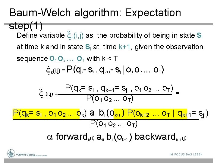
Baum-Welch algorithm: Expectation step(1) Define variable k(i, j) as the probability of being in state si at time k and in state sj at time k+1, given the observation sequence o 1 o 2. . . o with k < T (i, j) = P(q = s , q = s | o o. . . o ) k (i, j) = k T k i k+1 j 1 2 T P(qk= si , qk+1= sj , o 1 o 2. . . o. T) = P(o 1 o 2. . . o. T) P(qk= si , o 1 o 2. . . ok) aij bj (ok+1 ) P(ok+2. . . o. T | qk+1= sj ) = P(o 1 o 2. . . o. T) forward (i) a b (o ) backward k ij j k+1(j)
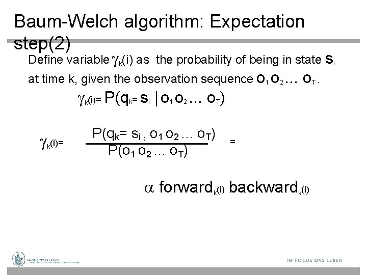
Baum-Welch algorithm: Expectation step(2) Define variable k(i) as the probability of being in state si at time k, given the observation sequence o 1 o 2. . . o (i)= P(q = s | o o. . . o ) k (i)= k k i 1 2 T P(qk= si , o 1 o 2. . . o. T) P(o 1 o 2. . . o. T) = forward (i) backward (i) k k T.
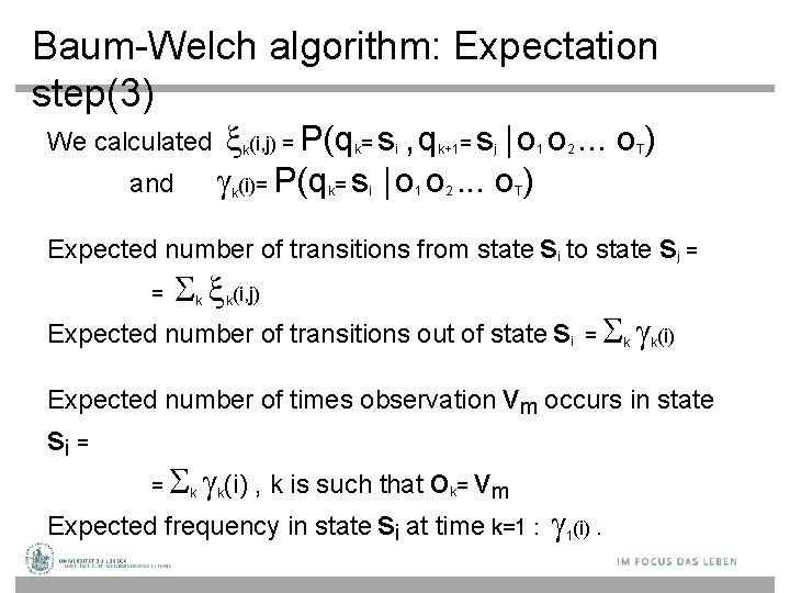
Baum-Welch algorithm: Expectation step(3) We calculated and (i, j) = P(q = s , q = s | o o. . . o ) (i)= P(q = s | o o. . . o ) k k i i k+1 1 2 j 1 2 T T Expected number of transitions from state si to state sj = = (i, j) k k Expected number of transitions out of state si = (i) k k Expected number of times observation vm occurs in state si = (i) , k is such that o = vm Expected frequency in state si at time k=1 : (i). = k k k 1
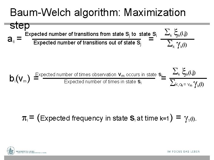
Baum-Welch algorithm: Maximization step a= ij k = m k k k (i, j) = k, o = v (i) Expected number of times observation vm occurs in state si Expected number of times in state si b (v ) = i (i, j) (i) Expected number of transitions from state sj to state si Expected number of transitions out of state sj k k k m = (Expected frequency in state s at time k=1) = (i). i i 1 k
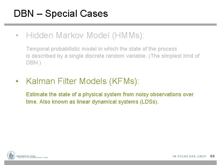
DBN – Special Cases • Hidden Markov Model (HMMs): Temporal probabilistic model in which the state of the process is described by a single discrete random variable. (The simplest kind of DBN ) • Kalman Filter Models (KFMs): Estimate the state of a physical system from noisy observations over time. Also known as linear dynamical systems (LDSs). 69
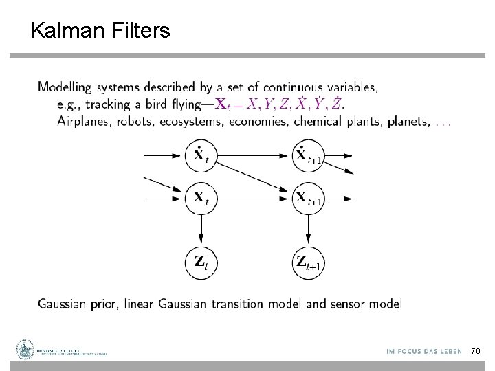
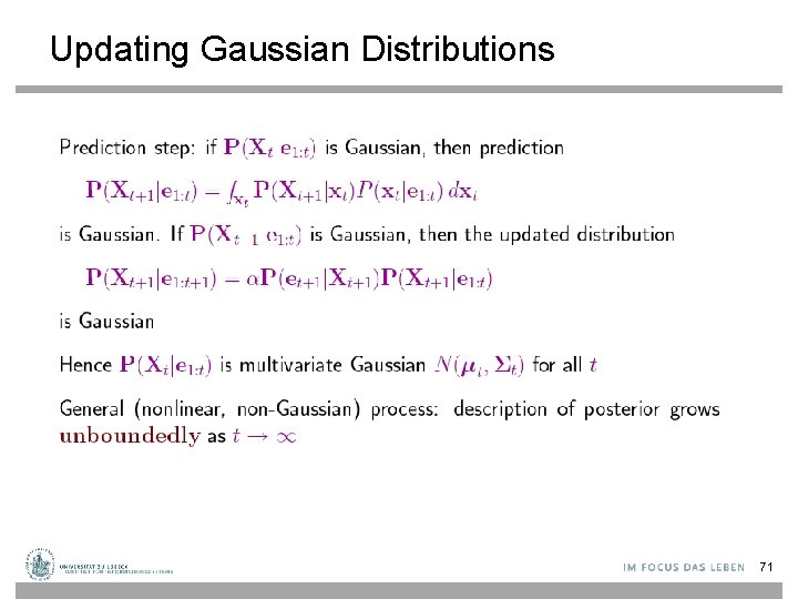
Kalman Filters 70
Updating Gaussian Distributions 71
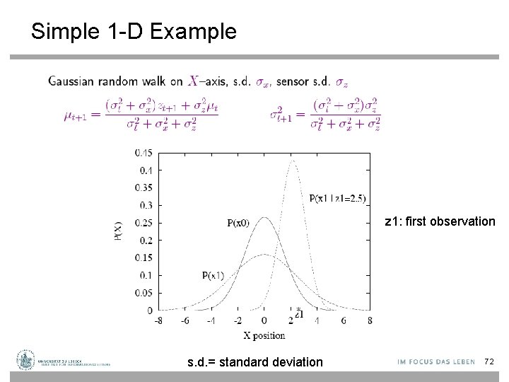
Simple 1 -D Example z 1: first observation s. d. = standard deviation 72
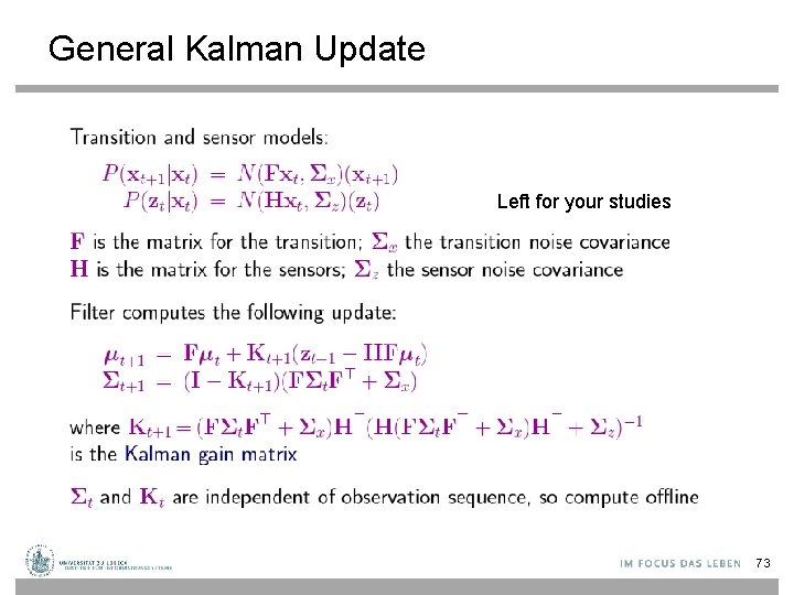
General Kalman Update Left for your studies 73
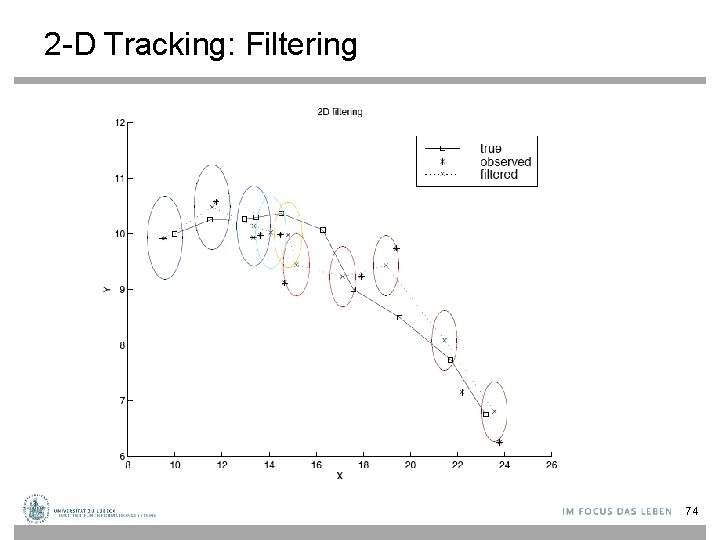
2 -D Tracking: Filtering 74
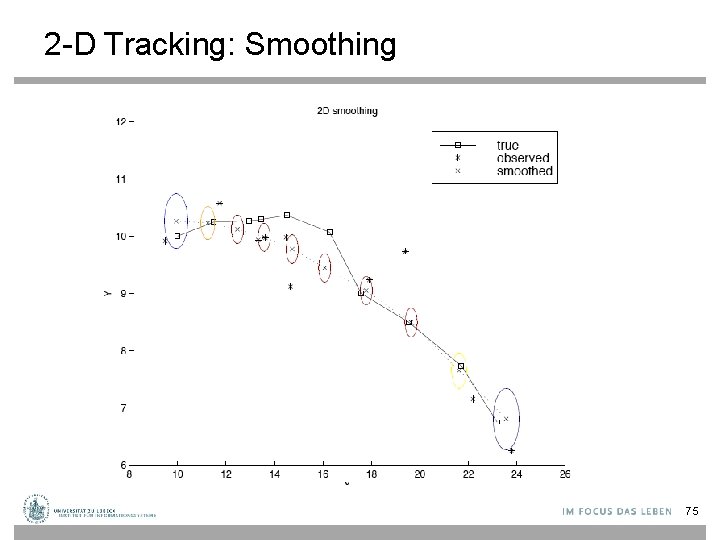
2 -D Tracking: Smoothing 75
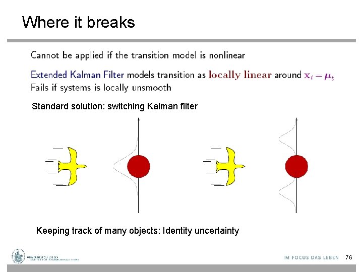
Where it breaks Standard solution: switching Kalman filter Keeping track of many objects: Identity uncertainty 76
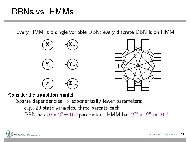
DBNs vs. HMMs Consider the transition model 77
Learning (1) • • The techniques for learning DBN are mostly straightforward extensions of the techniques for learning BNs Parameter learning – The transition model P(Xt | Xt-1) / The observation model P(Yt | Xt) – Offline learning • Parameters must be tied across time-slices • The initial state of the dynamic system can be learned independently of the transition matrix – Online learning • Add the parameters to the state space and then do online inference (filtering) – The usual criterion is maximum-likelihood(ML) • The goal of parameter learning is to compute – θ*ML = argmaxθP( Y| θ) = argmaxθlog P( Y| θ) – θ*MAP = argmaxθlog P( Y| θ) + log. P(θ) – Two standard approaches: gradient ascent and EM(Expectation Maximization) 78/29
Learning (2) • Structure learning – Intra-slice connectivity: Structural EM – Inter-slice connectivity: For each node in slice t, we must choose its parents from slice t-1 – Given structure is unrolled to a certain extent, the inter-slice connectivity is identical for all pairs of slices: • Constraints on Structural EM 79/29
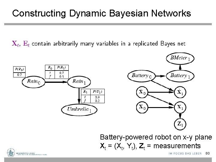
Constructing Dynamic Bayesian Networks Battery-powered robot on x-y plane Xt = (Xt, Yt), Zt = measurements 80
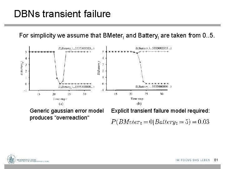
DBNs transient failure For simplicity we assume that BMetert and Batteryt are taken from 0. . 5. Generic gaussian error model produces “overreaction“ Explicit transient failure model required: 81
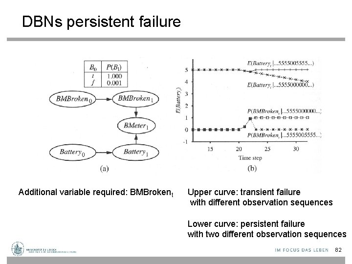
DBNs persistent failure Additional variable required: BMBrokent Upper curve: transient failure with different observation sequences Lower curve: persistent failure with two different observation sequences 82
- Slides: 82