NonStandard Databases and Data Mining Counterfactuals Dr zgr

Non-Standard Databases and Data Mining Counterfactuals Dr. Özgür Özçep Universität zu Lübeck Institut für Informationssysteme Presented by Prof. Dr. Ralf Möller

Structural Causal Models slides prepared by Özgür Özçep Part IV: Counterfactuals

Literature • J. Pearl, M. Glymour, N. P. Jewell: Causal inference in statistics – A primer, Wiley, 2016. (Main Reference) • J. Pearl: Causality, CUP, 2000. 3
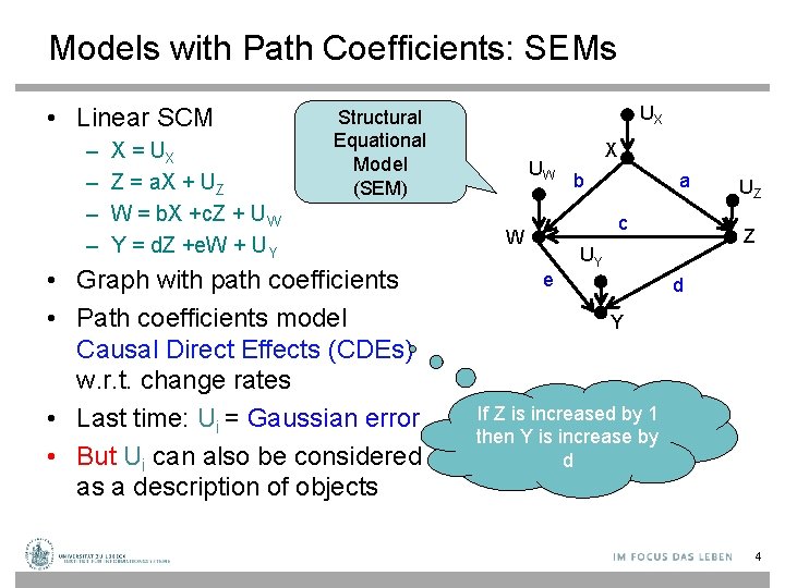
Models with Path Coefficients: SEMs • Linear SCM – – X = UX Z = a. X + UZ W = b. X +c. Z + UW Y = d. Z +e. W + UY UX Structural Equational Model (SEM) • Graph with path coefficients • Path coefficients model Causal Direct Effects (CDEs) w. r. t. change rates • Last time: Ui = Gaussian error • But Ui can also be considered as a description of objects UW X b a c W e UZ Z UY d Y If Z is increased by 1 then Y is increase by d 4
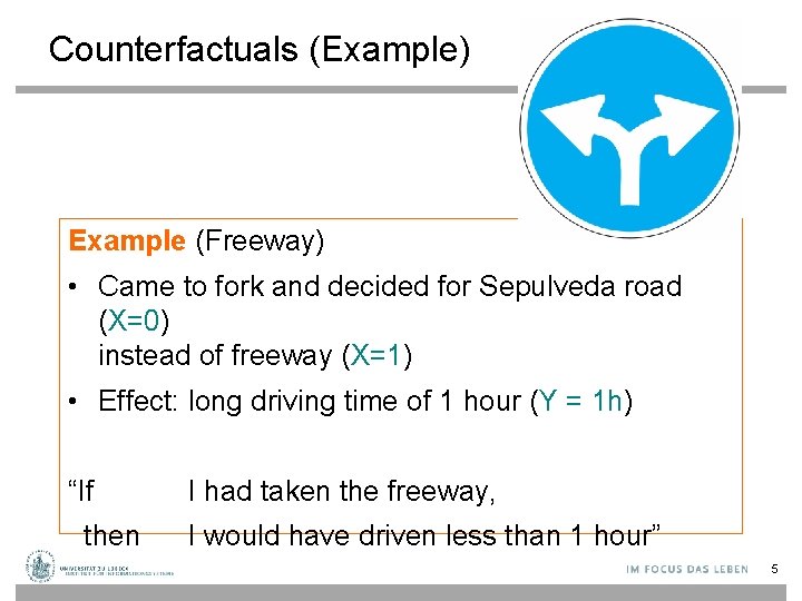
Counterfactuals (Example) Example (Freeway) • Came to fork and decided for Sepulveda road (X=0) instead of freeway (X=1) • Effect: long driving time of 1 hour (Y = 1 h) “If then I had taken the freeway, I would have driven less than 1 hour” 5
Counterfactuals (Informal Definition) Definition A counterfactual is an if-then statement where: – the if-condition, aka antecedent, hypothesizes about an alternative non-actual situation/condition (in example: taking freeway) and – then-condition, aka succedent, describes some consequence of the hypothetical situation (in example: less than 1 h drive) 6
Counterfactuals ≠ truth-conditional if • Counterfactuals may be false even if antecedent is false – “If Hamburg is capital of Germany, then Udo Lindenberg is chancellor” true – “If Hamburg had been capital of Germany then Udo Lindenberg would have been chancellor” false • Usually, in natural language use, the antecedent in counterfactuals is false in actual world • In natural language distinguished by different modes – indicative mode for truth-conditional if-statements vs. – conjunctive/subjunctive for counterfactuals 7
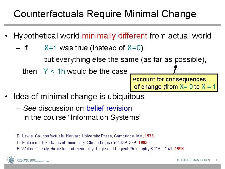
Counterfactuals Require Minimal Change • Hypothetical world minimally different from actual world – If X=1 was true (instead of X=0), but everything else the same (as far as possible), then Y < 1 h would be the case Account for consequences of change (from X= 0 to X = 1). • Idea of minimal change is ubiquitous – See discussion on belief revision in the course “Information Systems” D. Lewis. Counterfactuals. Harvard University Press, Cambridge, MA, 1973. D. Makinson. Five faces of minimality. Studia Logica, 52: 339– 379, 1993. F. Wolter. The algebraic face of minimality. Logic and Logical Philosophy, 6: 225 – 240, 1998. 8
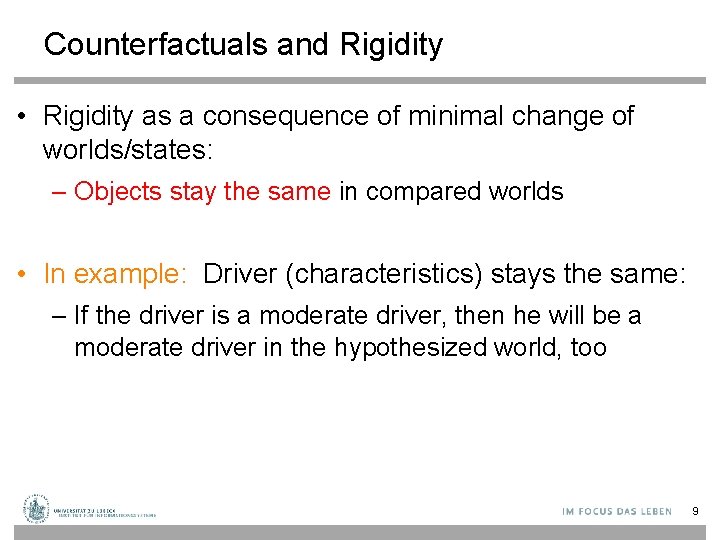
Counterfactuals and Rigidity • Rigidity as a consequence of minimal change of worlds/states: – Objects stay the same in compared worlds • In example: Driver (characteristics) stays the same: – If the driver is a moderate driver, then he will be a moderate driver in the hypothesized world, too 9
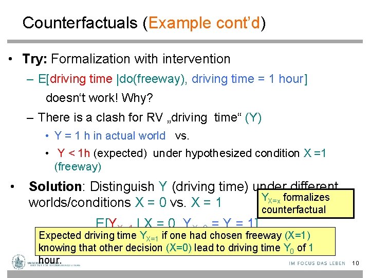
Counterfactuals (Example cont’d) • Try: Formalization with intervention – E[driving time |do(freeway), driving time = 1 hour] doesn‘t work! Why? – There is a clash for RV „driving time“ (Y) • Y = 1 h in actual world vs. • Y < 1 h (expected) under hypothesized condition X =1 (freeway) • Solution: Distinguish Y (driving time) under different YX=x formalizes worlds/conditions X = 0 vs. X = 1 counterfactual E[YX=1 | X = 0, YX=0 = Y = 1] Expected driving time YX=1 if one had chosen freeway (X=1) knowing that other decision (X=0) lead to driving time Y 0 of 1 hour. 10
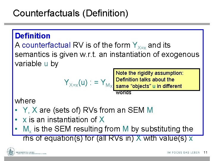
Counterfactuals (Definition) Definition A counterfactual RV is of the form YX=x and its semantics is given w. r. t. an instantiation of exogenous variable u by YX=x(u) : = Note the rigidity assumption: Definition talks about the YMx(u) same “objects” u in different worlds where • Y, X are (sets of) RVs from an SEM M • x is an instantiation of X • Mx is the SEM resulting from M by substituting the rhs of equation(s) for (all RVs in) X with value(s) x 11
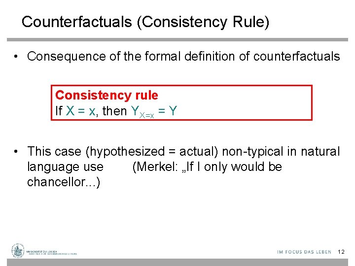
Counterfactuals (Consistency Rule) • Consequence of the formal definition of counterfactuals Consistency rule If X = x, then YX=x = Y • This case (hypothesized = actual) non-typical in natural language use (Merkel: „If I only would be chancellor. . . ) 12
Counterfactuals (for Linear SEMs) • How to formalize semantics of counterfactuals? – Use ideas similar to those of intervention • Consider linear models – Values of all variables determined by values of exogenous variables U = U 1, . . . , Un – So can write X = X(U) for any variable in SEM – Example • X: Salary, u = u 1, . . . , un characterizes individual Joe • X(u) = Joe‘s salary – When considering different worlds, the individuals (such as Joe = (u 1, . . . , un)) stay the same. 13

Counterfactuals in linear SEMs (Example) • Linear model M: X = a. U ; Y = b. X + U • Find YX=x(u) = ? (value of Y if it were the case that X = x for individual u) • Algorithm 1. Identify u under evidence (here: u just given) 2. Consider modified model Mx • X=x • Y = b. X + U 3. Calculate YX=x(u) = bx + u 14
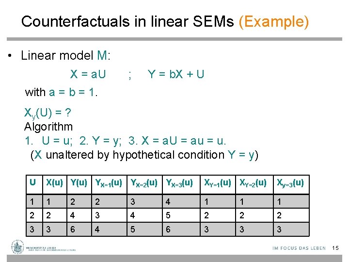
Counterfactuals in linear SEMs (Example) • Linear model M: X = a. U ; Y = b. X + U with a = b = 1. Xy(U) = ? Algorithm 1. U = u; 2. Y = y; 3. X = a. U = au = u. (X unaltered by hypothetical condition Y = y) U X(u) YX=1(u) YX=2(u) YX=3(u) XY=1(u) XY=2(u) Xy=3(u) 1 1 2 2 3 4 1 1 1 2 2 4 3 4 5 2 2 2 3 3 6 4 5 6 3 3 3 15
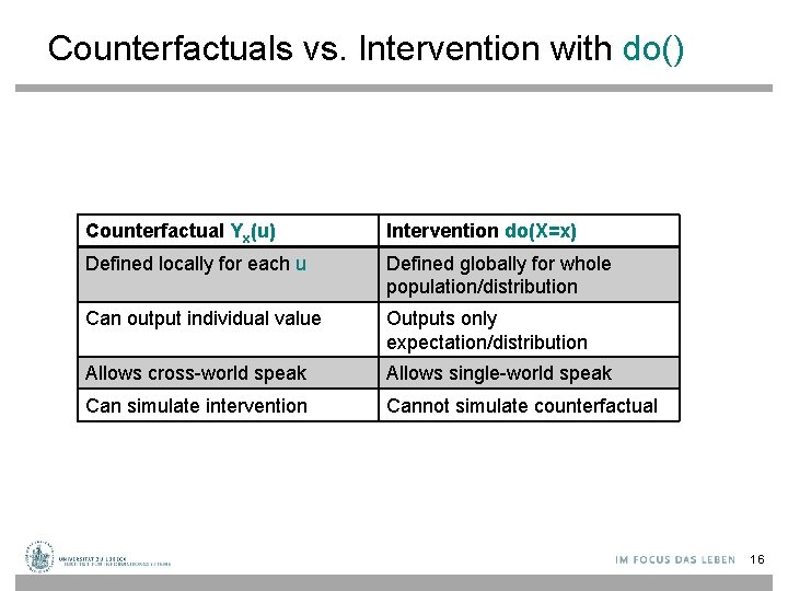
Counterfactuals vs. Intervention with do() Counterfactual Yx(u) Intervention do(X=x) Defined locally for each u Defined globally for whole population/distribution Can output individual value Outputs only expectation/distribution Allows cross-world speak Allows single-world speak Can simulate intervention Cannot simulate counterfactual 16
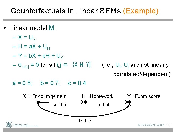
Counterfactuals in Linear SEMs (Example) • Linear model M: – X = UX – H = a. X + UH – Y = b. X + c. H + UY – σUi. Uj = 0 for all i, j ∈ {X, H, Y} (i. e. , Ui, Uj are not linearly correlated/dependent) a = 0. 5; b = 0. 7; X = Encouragement c = 0. 4 H= Homework a=0. 5 Y= Exam score c=0. 4 b=0. 7 17
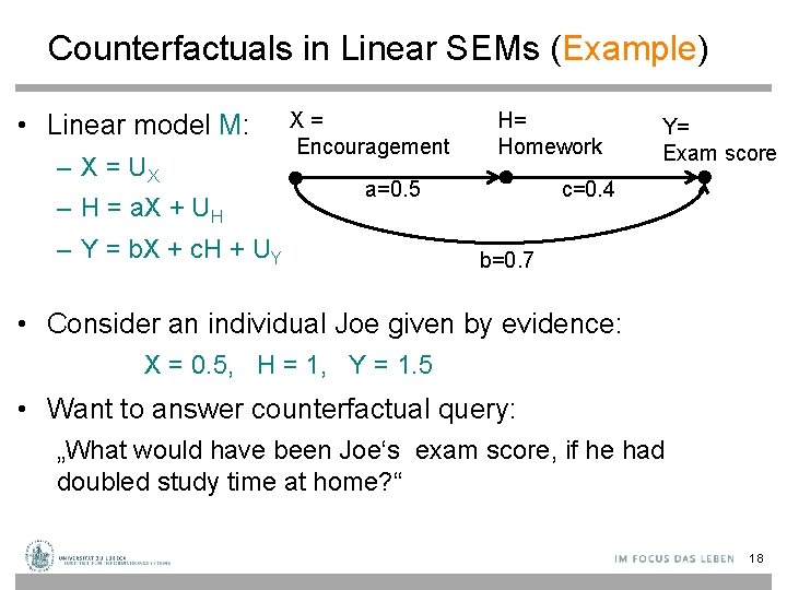
Counterfactuals in Linear SEMs (Example) • Linear model M: – X = UX – H = a. X + UH X= Encouragement H= Homework a=0. 5 – Y = b. X + c. H + UY Y= Exam score c=0. 4 b=0. 7 • Consider an individual Joe given by evidence: X = 0. 5, H = 1, Y = 1. 5 • Want to answer counterfactual query: „What would have been Joe‘s exam score, if he had doubled study time at home? “ 18
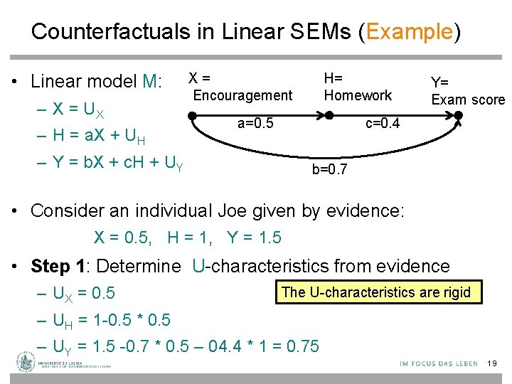
Counterfactuals in Linear SEMs (Example) • Linear model M: – X = UX – H = a. X + UH X= Encouragement H= Homework a=0. 5 Y= Exam score c=0. 4 – Y = b. X + c. H + UY b=0. 7 • Consider an individual Joe given by evidence: X = 0. 5, H = 1, Y = 1. 5 • Step 1: Determine U-characteristics from evidence – UX = 0. 5 The U-characteristics are rigid – UH = 1 -0. 5 * 0. 5 – UY = 1. 5 -0. 7 * 0. 5 – 04. 4 * 1 = 0. 75 19
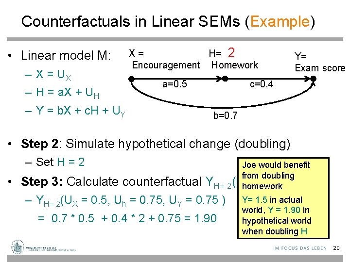
Counterfactuals in Linear SEMs (Example) • Linear model M: – X = UX – H = a. X + UH X= H= 2 Encouragement Homework a=0. 5 – Y = b. X + c. H + UY Y= Exam score c=0. 4 b=0. 7 • Step 2: Simulate hypothetical change (doubling) – Set H = 2 • Step 3: Calculate counterfactual Joe would benefit from doubling YH= 2(u)homework – YH= 2(UX = 0. 5, Uh = 0. 75, UY = 0. 75 ) = 0. 7 * 0. 5 + 0. 4 * 2 + 0. 75 = 1. 90 Y= 1. 5 in actual world, Y = 1. 90 in hypothetical world when doubling H 20
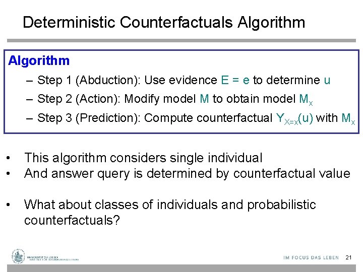
Deterministic Counterfactuals Algorithm – Step 1 (Abduction): Use evidence E = e to determine u – Step 2 (Action): Modify model M to obtain model Mx – Step 3 (Prediction): Compute counterfactual YX=x(u) with Mx • • This algorithm considers single individual And answer query is determined by counterfactual value • What about classes of individuals and probabilistic counterfactuals? 21
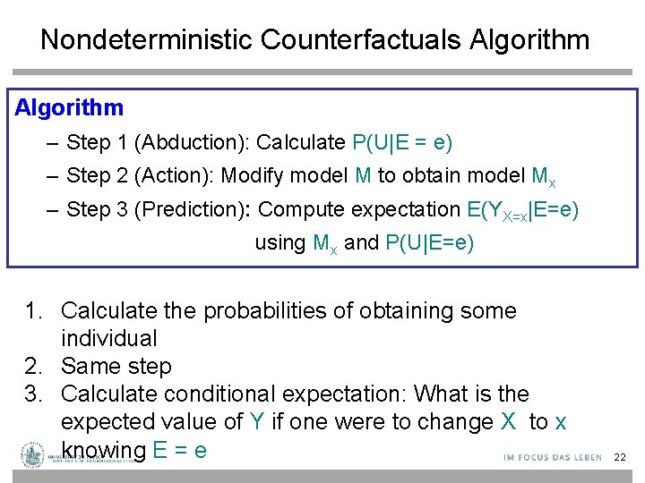
Nondeterministic Counterfactuals Algorithm – Step 1 (Abduction): Calculate P(U|E = e) – Step 2 (Action): Modify model M to obtain model Mx – Step 3 (Prediction): Compute expectation E(YX=x|E=e) using Mx and P(U|E=e) 1. Calculate the probabilities of obtaining some individual 2. Same step 3. Calculate conditional expectation: What is the expected value of Y if one were to change X to x knowing E = e 22
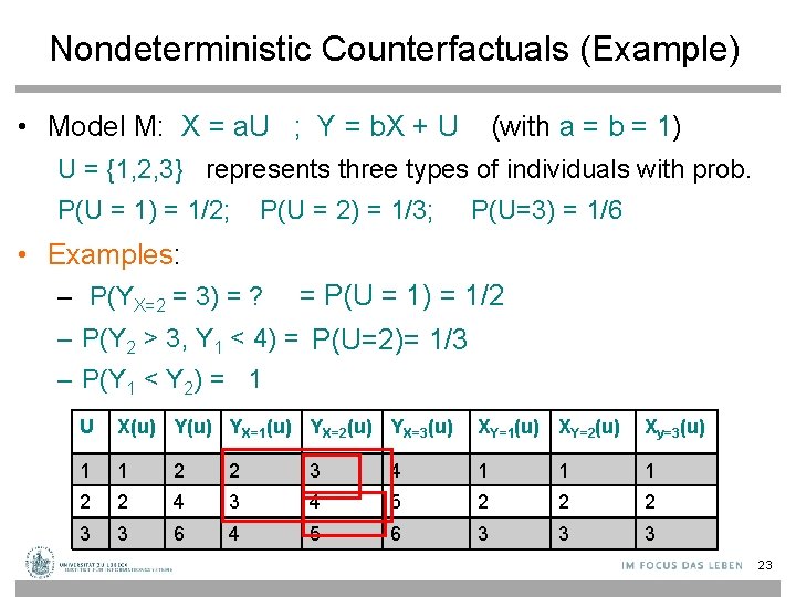
Nondeterministic Counterfactuals (Example) • Model M: X = a. U ; Y = b. X + U (with a = b = 1) U = {1, 2, 3} represents three types of individuals with prob. P(U = 1) = 1/2; P(U = 2) = 1/3; P(U=3) = 1/6 • Examples: – P(YX=2 = 3) = ? = P(U = 1) = 1/2 – P(Y 2 > 3, Y 1 < 4) = P(U=2)= 1/3 – P(Y 1 < Y 2) = 1 U X(u) YX=1(u) YX=2(u) YX=3(u) XY=1(u) XY=2(u) Xy=3(u) 1 1 2 2 3 4 1 1 1 2 2 4 3 4 5 2 2 2 3 3 6 4 5 6 3 3 3 23
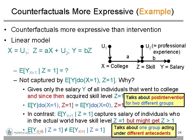
Counterfactuals More Expressive (Example) • Counterfactuals more expressive than intervention • Linear model X = U 1; Z = a. X + U 2; Y = b. Z – E[YX=1 | Z = 1] = ? U 1 a X = College U 2 (= professional experience) b Z = Skill Y = Salary – Not captured by E[Y|do(X=1), Z=1]. Why? • Gives only the salary Y of all individuals that went to college and since then acquired skill level Z=1. Talks about postintervention • E[Y|do(X=1), Z=1] = E[Y|do(X=0), Z=1]for two different groups • In contrast: E[YX=1 | Z = 1] captures salary of individuals who in the actual world have skill level Z =1 but might get Z > 1 • E[YX=0 | Z = 1] ≠ E[YX=1 | Z = 1] Talks about one group acting under different antecedents 24
![Counterfactuals More Expressive (Example) • E[YX=0 | Z = 1] ≠ E[YX=1 | Z Counterfactuals More Expressive (Example) • E[YX=0 | Z = 1] ≠ E[YX=1 | Z](http://slidetodoc.com/presentation_image_h2/27dd739acb43c3573a009c90751ad973/image-25.jpg)
Counterfactuals More Expressive (Example) • E[YX=0 | Z = 1] ≠ E[YX=1 | Z = 1]? U 1 – How is this reflected in numbers? a b X = College Z = Skill Y = Salary – Later: How reflected in graph? X = U 1; Z = a. X + U 2; Y = b. Z U 2 (for a ≠ 1 and a ≠ 0, b≠ 0) u 1 u 2 X(u) Z(u) YX=0(u) YX=1(u) ZX=0(u) ZX=1(u) 0 0 0 ab 0 a 0 1 b b (a+1)b 1 a+1 1 0 1 a ab 0 a 1 1 1 a+1 (a+1)b b (a+1)b 1 a+1 • E[Y 1|Z=1] = (a+1)b • E[Y 0|Z=1] = b ; E[Y|do(X=1), Z=1] = b ; E[Y|do(X=0), Z=1] = b In particular: E[Y 1 -Y 0|Z=1] = ab ≠ 0 25
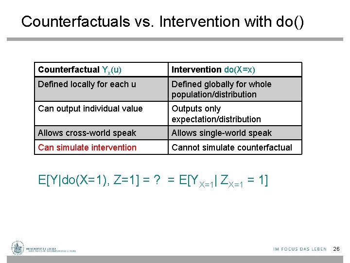
Counterfactuals vs. Intervention with do() Counterfactual Yx(u) Intervention do(X=x) Defined locally for each u Defined globally for whole population/distribution Can output individual value Outputs only expectation/distribution Allows cross-world speak Allows single-world speak Can simulate intervention Cannot simulate counterfactual E[Y|do(X=1), Z=1] = ? = E[YX=1| ZX=1 = 1] 26
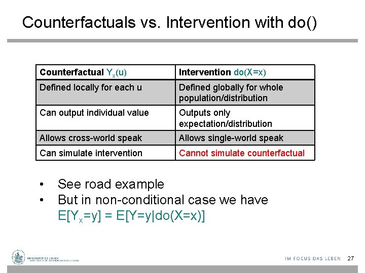
Counterfactuals vs. Intervention with do() Counterfactual Yx(u) Intervention do(X=x) Defined locally for each u Defined globally for whole population/distribution Can output individual value Outputs only expectation/distribution Allows cross-world speak Allows single-world speak Can simulate intervention Cannot simulate counterfactual • • See road example But in non-conditional case we have E[Yx=y] = E[Y=y|do(X=x)] 27
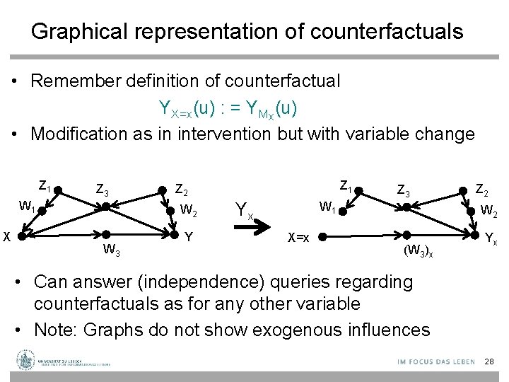
Graphical representation of counterfactuals • Remember definition of counterfactual YX=x(u) : = YMx(u) • Modification as in intervention but with variable change Z 1 Z 3 W 1 X W 2 W 3 Z 1 Z 2 Y Yx Z 3 W 1 X=x Z 2 W 2 (W 3)x Yx • Can answer (independence) queries regarding counterfactuals as for any other variable • Note: Graphs do not show exogenous influences 28
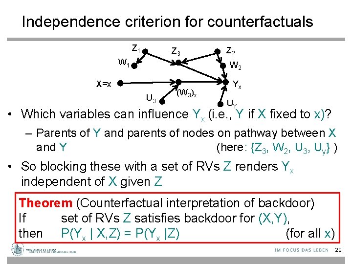
Independence criterion for counterfactuals Z 1 Z 3 W 1 Z 2 W 2 X=x U 3 (W 3)x Yx UY • Which variables can influence Yx (i. e. , Y if X fixed to x)? – Parents of Y and parents of nodes on pathway between X and Y (here: {Z 3, W 2, U 3, Uy} ) • So blocking these with a set of RVs Z renders Yx independent of X given Z Theorem (Counterfactual interpretation of backdoor) If set of RVs Z satisfies backdoor for (X, Y), then P(Yx | X, Z) = P(Yx |Z) (for all x) 29
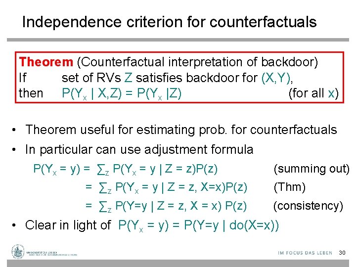
Independence criterion for counterfactuals Theorem (Counterfactual interpretation of backdoor) If set of RVs Z satisfies backdoor for (X, Y), then P(Yx | X, Z) = P(Yx |Z) (for all x) • Theorem useful for estimating prob. for counterfactuals • In particular can use adjustment formula P(Yx = y) = ∑z P(Yx = y | Z = z)P(z) (summing out) = ∑z P(Yx = y | Z = z, X=x)P(z) (Thm) = ∑z P(Y=y | Z = z, X = x) P(z) (consistency) • Clear in light of P(Yx = y) = P(Y=y | do(X=x)) 30
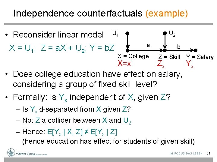
Independence counterfactuals (example) • Reconsider linear model U 1 X = U 1; Z = a. X + U 2; Y = b. Z U 2 a X = College X=x b Z = Skill Y = Salary Zx • Does college education have effect on salary, considering a group of fixed skill level? Yx • Formally: Is Yx independent of X, given Z? – Is Yx d-separated from X given Z? – No: Z a collider between X and U 2 – Hence: E[Yx | X, Z] ≠ E[Yx | Z] (hence education has effect for students of given skill) 31
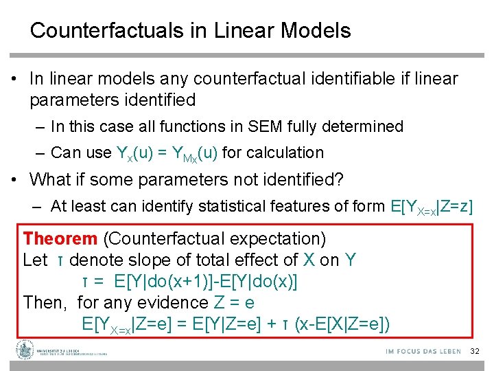
Counterfactuals in Linear Models • In linear models any counterfactual identifiable if linear parameters identified – In this case all functions in SEM fully determined – Can use Yx(u) = YMx(u) for calculation • What if some parameters not identified? – At least can identify statistical features of form E[YX=x|Z=z] Theorem (Counterfactual expectation) Let τ denote slope of total effect of X on Y τ = E[Y|do(x+1)]-E[Y|do(x)] Then, for any evidence Z = e E[YX=x|Z=e] = E[Y|Z=e] + τ (x-E[X|Z=e]) 32
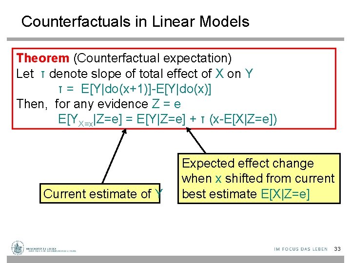
Counterfactuals in Linear Models Theorem (Counterfactual expectation) Let τ denote slope of total effect of X on Y τ = E[Y|do(x+1)]-E[Y|do(x)] Then, for any evidence Z = e E[YX=x|Z=e] = E[Y|Z=e] + τ (x-E[X|Z=e]) Current estimate of Y Expected effect change when x shifted from current best estimate E[X|Z=e] 33
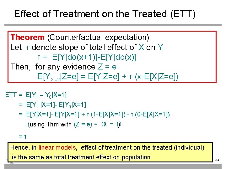
Effect of Treatment on the Treated (ETT) Theorem (Counterfactual expectation) Let τ denote slope of total effect of X on Y τ = E[Y|do(x+1)]-E[Y|do(x)] Then, for any evidence Z = e E[YX=x|Z=e] = E[Y|Z=e] + τ (x-E[X|Z=e]) ETT = E[Y 1 – Y 0|X=1] = E[Y 1 |X=1]- E[Y 0|X=1] = E[Y|X=1]- E[Y|X=1] + τ (1 -E[X|X=1]) - τ (0 -E[X|X=1]) (using Thm with (Z = e) ≙ (X = 1) ) =τ Hence, in linear models, effect of treatment on the treated (individual) is the same as total treatment effect on population 34
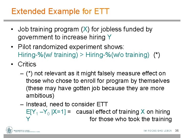
Extended Example for ETT • Job training program (X) for jobless funded by government to increase hiring Y • Pilot randomized experiment shows: Hiring-%(w/ training) > Hiring-%(w/o training) (*) • Critics – (*) not relevant as it might falsely measure effect on those who chose to enroll for program by themselves (these may have gotten job because they are more ambitious) – Instead, need to consider ETT E[Y 1 –Y 0 |X=1] = causal effect of training X on hiring Y for those who took the training 35
![Extended Example for ETT (cont’d) • Difficult part: E[YX=0 |X=1] – not given by Extended Example for ETT (cont’d) • Difficult part: E[YX=0 |X=1] – not given by](http://slidetodoc.com/presentation_image_h2/27dd739acb43c3573a009c90751ad973/image-36.jpg)
Extended Example for ETT (cont’d) • Difficult part: E[YX=0 |X=1] – not given by observational or experimental data – but can be reduced to these if appropriate covariates Z (fulfilling backdoor criterion) exist P(Yx = y | X = x‘) = ∑z P(Yx = y | Z = z, x‘)P(z|x‘) = ∑z P(Yx = y | Z = z, x)P(z|x‘) (by condition on z) (by Thm on counterfactual backdoor P(Yx | X, Z) = P(Yx |Z) ) = ∑z P(Y = y | Z = z, x)P(z|x‘) (consistency rule) Contains only observational/testable RVs • E[Y 0|X=1] = ∑z E(Y | Z = z, X=0)P(z|X=1) (after substitution and commuting sums) 36
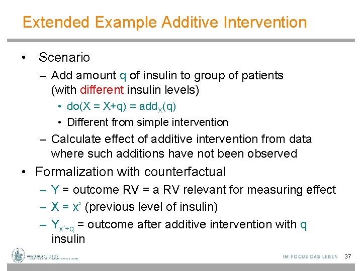
Extended Example Additive Intervention • Scenario – Add amount q of insulin to group of patients (with different insulin levels) • do(X = X+q) = add. X(q) • Different from simple intervention – Calculate effect of additive intervention from data where such additions have not been observed • Formalization with counterfactual – Y = outcome RV = a RV relevant for measuring effect – X = x’ (previous level of insulin) – Yx‘+q = outcome after additive intervention with q insulin 37
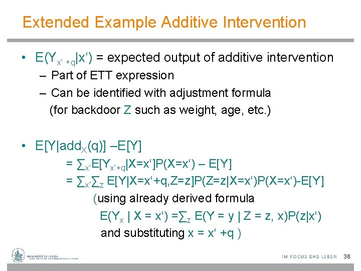
Extended Example Additive Intervention • E(Yx‘ +q|x‘) = expected output of additive intervention – Part of ETT expression – Can be identified with adjustment formula (for backdoor Z such as weight, age, etc. ) • E[Y|add. X(q)] –E[Y] = ∑x‘E[Yx‘+q|X=x‘]P(X=x‘) – E[Y] = ∑x‘∑z E[Y|X=x‘+q, Z=z]P(Z=z|X=x‘)P(X=x‘)-E[Y] (using already derived formula E(Yx | X = x‘) =∑z E(Y = y | Z = z, x)P(z|x‘) and substituting x = x‘ +q ) 38
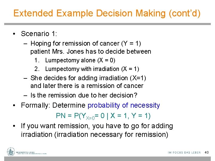
Extended Example Decision Making (cont’d) • Scenario 1: – Hoping for remission of cancer (Y = 1) patient Mrs. Jones has to decide between 1. Lumpectomy alone (X = 0) 2. Lumpectomy with irradiation (X = 1) – She decides for adding irradiation (X=1) and later there is a remission of cancer – Is the remission due to her decision? • Formally: Determine probability of necessity PN = P(YX=0= 0 | X = 1, Y = 1) • If you want remission, you have to go for adding irradiation (irradiation necessary for remission) 40
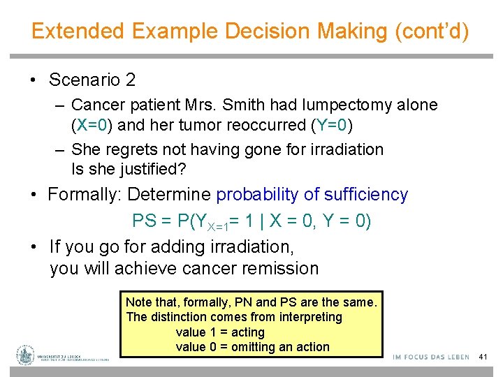
Extended Example Decision Making (cont’d) • Scenario 2 – Cancer patient Mrs. Smith had lumpectomy alone (X=0) and her tumor reoccurred (Y=0) – She regrets not having gone for irradiation Is she justified? • Formally: Determine probability of sufficiency PS = P(YX=1= 1 | X = 0, Y = 0) • If you go for adding irradiation, you will achieve cancer remission Note that, formally, PN and PS are the same. The distinction comes from interpreting value 1 = acting value 0 = omitting an action 41
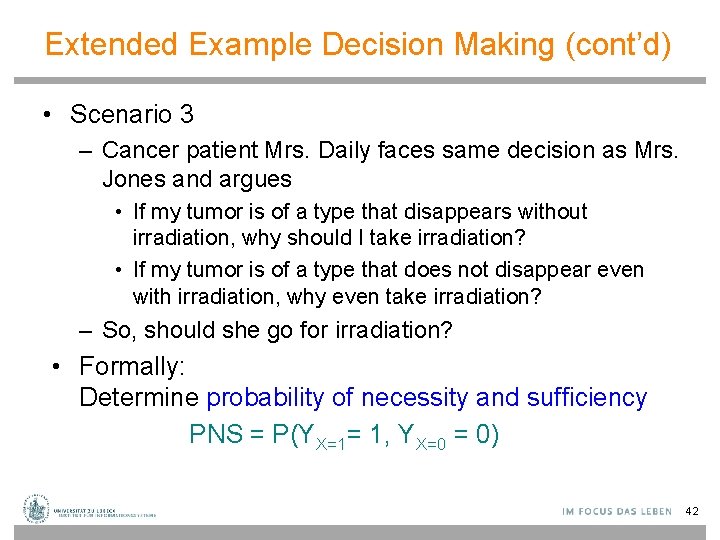
Extended Example Decision Making (cont’d) • Scenario 3 – Cancer patient Mrs. Daily faces same decision as Mrs. Jones and argues • If my tumor is of a type that disappears without irradiation, why should I take irradiation? • If my tumor is of a type that does not disappear even with irradiation, why even take irradiation? – So, should she go for irradiation? • Formally: Determine probability of necessity and sufficiency PNS = P(YX=1= 1, YX=0 = 0) 42
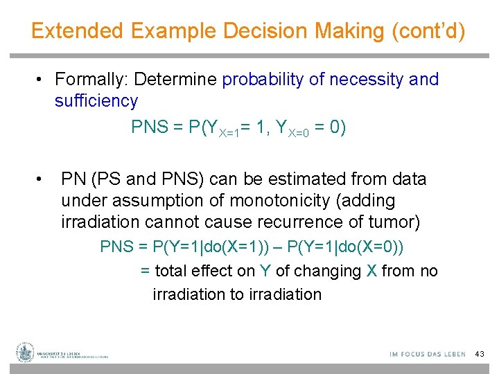
Extended Example Decision Making (cont’d) • Formally: Determine probability of necessity and sufficiency PNS = P(YX=1= 1, YX=0 = 0) • PN (PS and PNS) can be estimated from data under assumption of monotonicity (adding irradiation cannot cause recurrence of tumor) PNS = P(Y=1|do(X=1)) – P(Y=1|do(X=0)) = total effect on Y of changing X from no irradiation to irradiation 43
Summary • Counterfactual reasoning is not intervention – Can simulate intervention • Counterfactual reasoning required for certain applications – Compute the effect of different options – Reason about nessecity and sufficiency of diagnoses • Can do counterfactual reasoning in some cases even if models are incomplete 44
- Slides: 43