Nonparametric tests distributionfree tests Hypotheses Data transformation Data
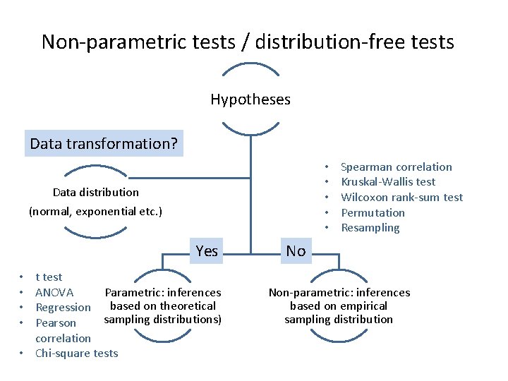
Non-parametric tests / distribution-free tests Hypotheses Data transformation? • • • Data distribution (normal, exponential etc. ) Yes t test Parametric: inferences ANOVA Regression based on theoretical sampling distributions) Pearson correlation • Chi-square tests • • Spearman correlation Kruskal-Wallis test Wilcoxon rank-sum test Permutation Resampling No Non-parametric: inferences based on empirical sampling distribution
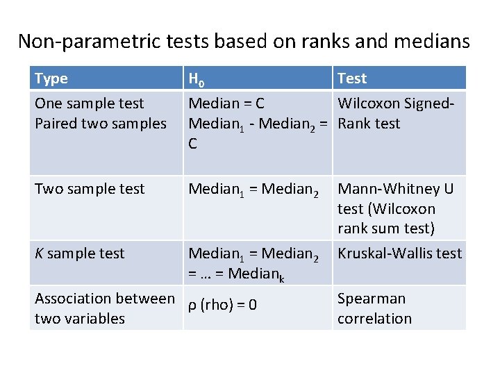
Non-parametric tests based on ranks and medians Type H 0 One sample test Paired two samples Median = C Wilcoxon Signed. Median 1 - Median 2 = Rank test C Two sample test Median 1 = Median 2 Mann-Whitney U test (Wilcoxon rank sum test) K sample test Median 1 = Median 2 = … = Mediank Kruskal-Wallis test Association between ρ (rho) = 0 two variables Test Spearman correlation
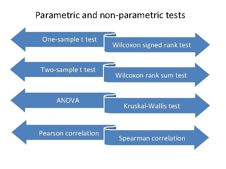
Parametric and non-parametric tests One-sample t test Two-sample t test ANOVA Pearson correlation Wilcoxon signed rank test Wilcoxon rank sum test Kruskal-Wallis test Spearman correlation
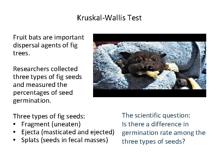
Kruskal-Wallis Test Fruit bats are important dispersal agents of fig trees. Researchers collected three types of fig seeds and measured the percentages of seed germination. Three types of fig seeds: • Fragment (uneaten) • Ejecta (masticated and ejected) • Splats (seeds in fecal masses) The scientific question: Is there a difference in germination rate among the three types of seeds?
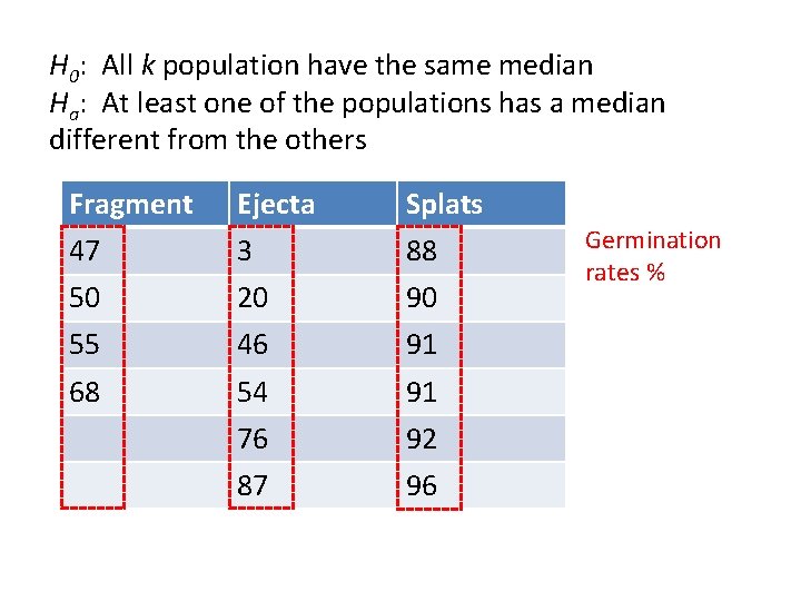
H 0: All k population have the same median Ha: At least one of the populations has a median different from the others Fragment Ejecta Splats 47 3 88 50 20 90 55 46 91 68 54 91 76 92 87 96 Germination rates %
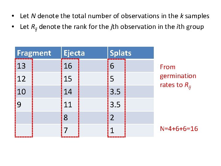
• Let N denote the total number of observations in the k samples • Let Rij denote the rank for the jth observation in the ith group Fragment Ejecta Splats 13 16 6 12 15 5 10 14 3. 5 9 11 3. 5 8 2 7 1 From germination rates to Rij N=4+6+6=16
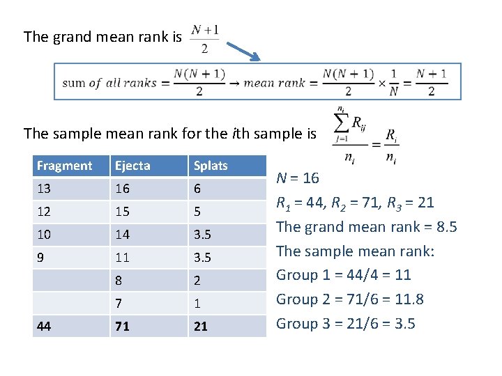
The grand mean rank is The sample mean rank for the ith sample is Fragment Ejecta Splats 13 16 6 12 15 5 10 14 3. 5 9 11 3. 5 8 2 7 1 71 21 44 N = 16 R 1 = 44, R 2 = 71, R 3 = 21 The grand mean rank = 8. 5 The sample mean rank: Group 1 = 44/4 = 11 Group 2 = 71/6 = 11. 8 Group 3 = 21/6 = 3. 5
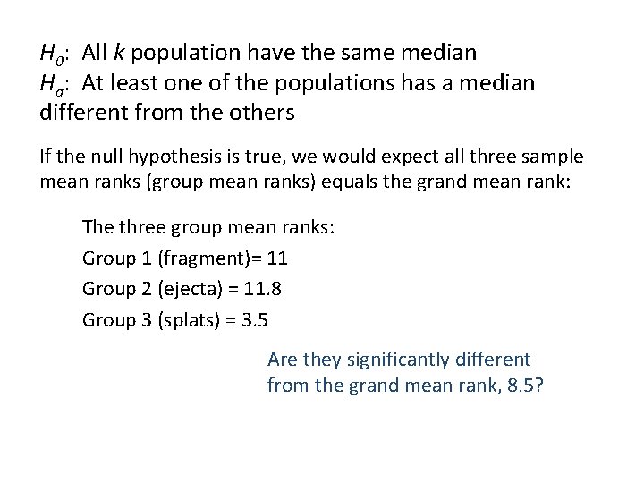
H 0: All k population have the same median Ha: At least one of the populations has a median different from the others If the null hypothesis is true, we would expect all three sample mean ranks (group mean ranks) equals the grand mean rank: The three group mean ranks: Group 1 (fragment)= 11 Group 2 (ejecta) = 11. 8 Group 3 (splats) = 3. 5 Are they significantly different from the grand mean rank, 8. 5?
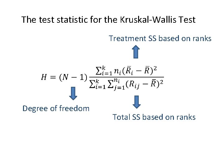
The test statistic for the Kruskal-Wallis Test Treatment SS based on ranks Degree of freedom Total SS based on ranks
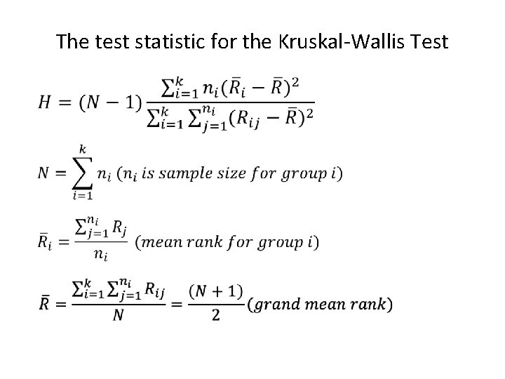
The test statistic for the Kruskal-Wallis Test
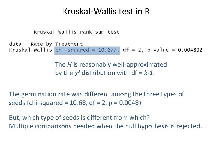
Kruskal-Wallis test in R The H is reasonably well-approximated by the χ2 distribution with df = k-1. The germination rate was different among the three types of seeds (chi-squared = 10. 68, df = 2, p = 0. 0048). But, which type of seeds is different from which? Multiple comparisons needed when the null hypothesis is rejected.
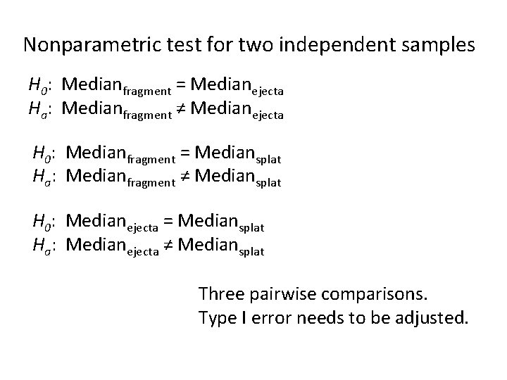
Nonparametric test for two independent samples H 0: Medianfragment = Medianejecta Ha: Medianfragment ≠ Medianejecta H 0: Medianfragment = Mediansplat Ha: Medianfragment ≠ Mediansplat H 0: Medianejecta = Mediansplat Ha: Medianejecta ≠ Mediansplat Three pairwise comparisons. Type I error needs to be adjusted.
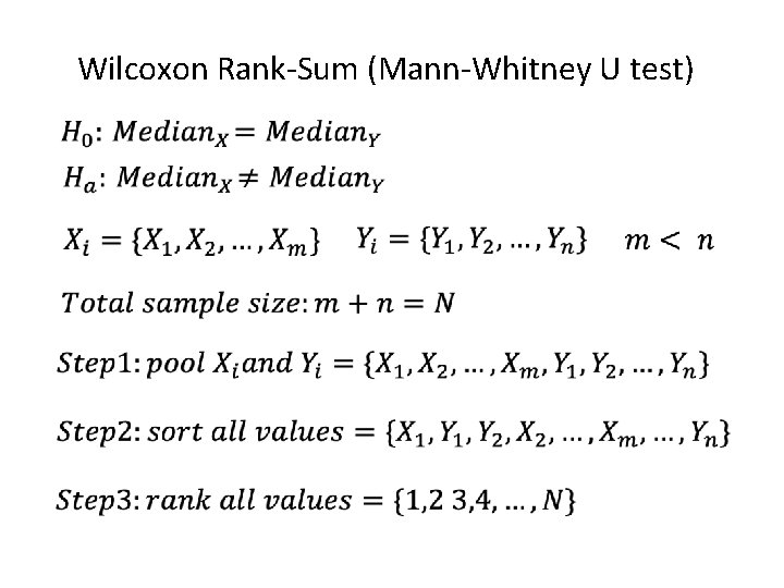
Wilcoxon Rank-Sum (Mann-Whitney U test)
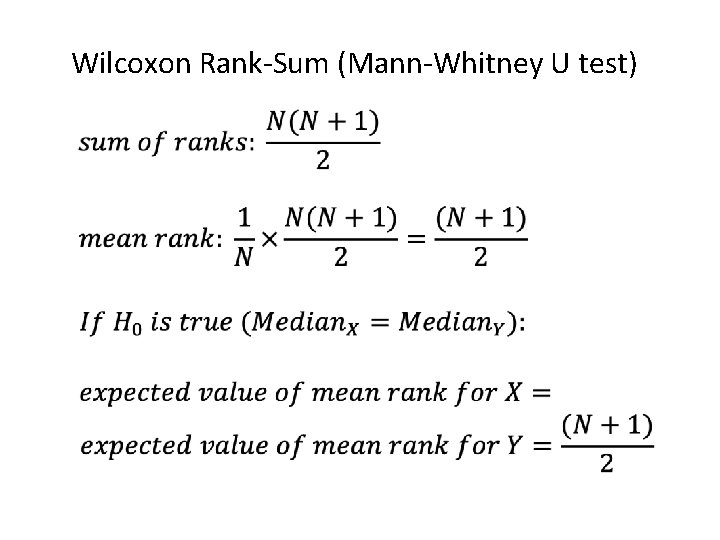
Wilcoxon Rank-Sum (Mann-Whitney U test)
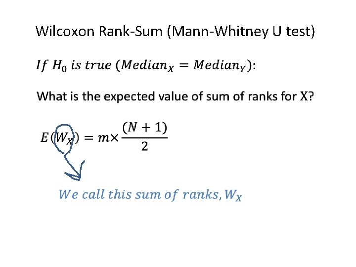
Wilcoxon Rank-Sum (Mann-Whitney U test)
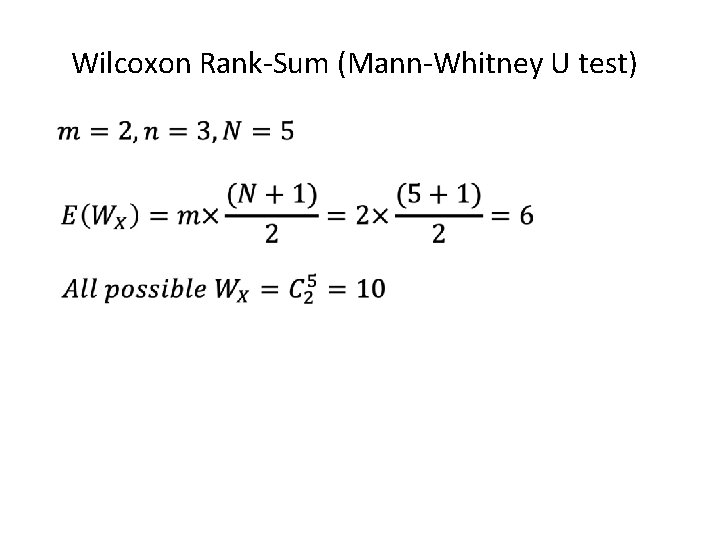
Wilcoxon Rank-Sum (Mann-Whitney U test)
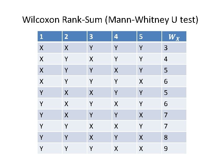
Wilcoxon Rank-Sum (Mann-Whitney U test) 1 X X X 2 X Y Y 3 Y X Y 4 Y Y X 5 Y Y Y 3 4 5 X Y Y Y Y X X X Y Y X X Y Y Y X Y X X Y Y X X 6 5 6 7 7 8 9
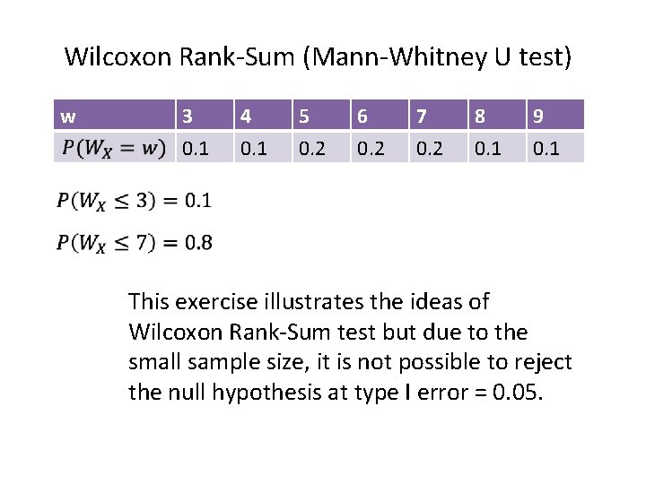
Wilcoxon Rank-Sum (Mann-Whitney U test) w 3 0. 1 4 0. 1 5 0. 2 6 0. 2 7 0. 2 8 0. 1 9 0. 1 This exercise illustrates the ideas of Wilcoxon Rank-Sum test but due to the small sample size, it is not possible to reject the null hypothesis at type I error = 0. 05.
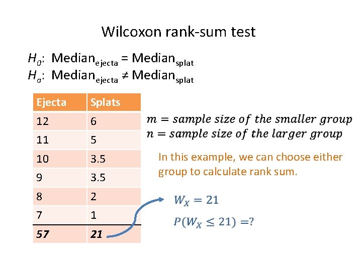
Wilcoxon rank-sum test H 0: Medianejecta = Mediansplat Ha: Medianejecta ≠ Mediansplat Ejecta Splats 12 6 11 5 10 3. 5 9 3. 5 8 2 7 1 57 21 In this example, we can choose either group to calculate rank sum.
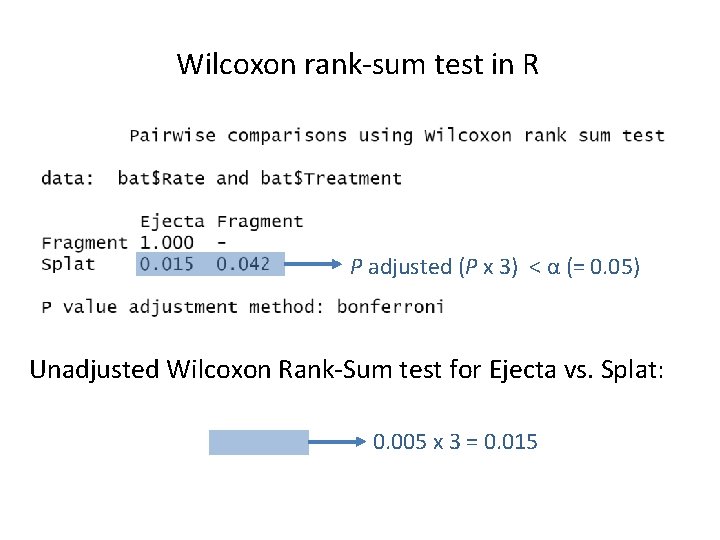
Wilcoxon rank-sum test in R P adjusted (P x 3) < α (= 0. 05) Unadjusted Wilcoxon Rank-Sum test for Ejecta vs. Splat: 0. 005 x 3 = 0. 015
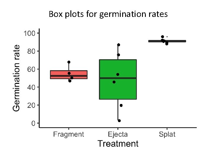
Box plots for germination rates
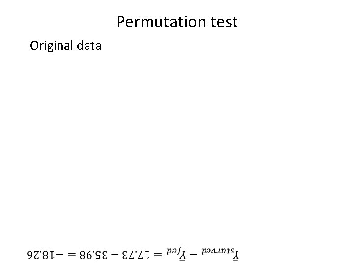
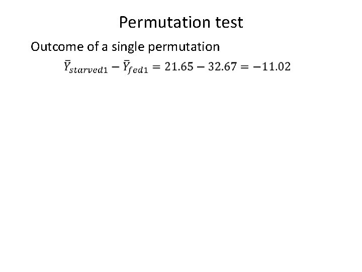
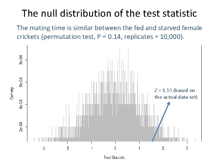
Permutation test Permutation means re-arrangement. In a permutation test, we take the values of the response variable and randomly re-arrange (permute) them across all levels of independent variables. This gives us an idea of what values the test statistic (such as t, χ2) would have if the two variables are not associated (i. e. null distribution). It makes no assumption about normality or equal variance.
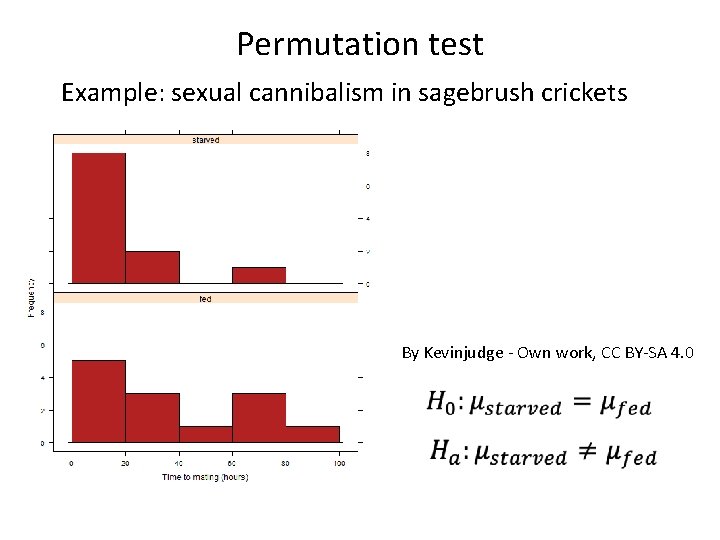
Permutation test Example: sexual cannibalism in sagebrush crickets By Kevinjudge - Own work, CC BY-SA 4. 0
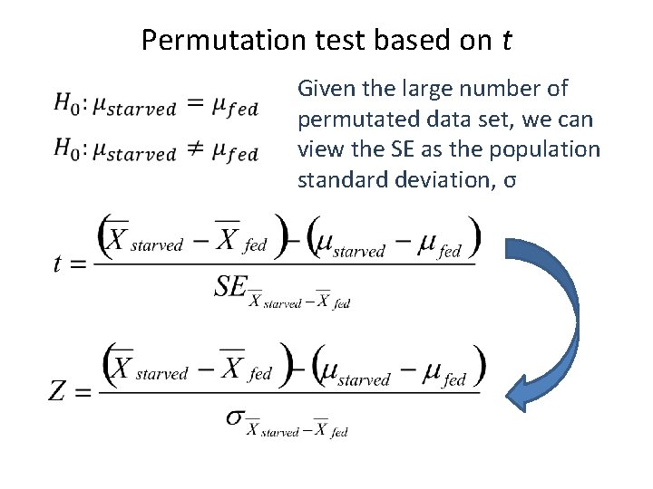
Permutation test based on t Given the large number of permutated data set, we can view the SE as the population standard deviation, σ
Permutation test Original data
Permutation test Outcome of a single permutation
The null distribution of the test statistic The mating time is similar between the fed and starved female crickets (permutation test, P = 0. 14, replicates = 10, 000). Z = 1. 53 (based on the actual data set)
Bootstrap CIs Bootstrap is a procedure used to approximate the sampling distribution of an estimate. Bootstrap creates this sampling distribution by resampling, taking new samples randomly and repeatedly from the data themselves. Simulation (such as permutation test) creates population distribution based on a specific hypothesis. It does not produce parameter estimates; it creates imaginary data sets. Bootstrap is very useful in providing means and confidence intervals for estimates with unknown distribution.
Bootstrap CIs The mean of the bootstrap replicates is the point estimate for whichever statistic, index or variable under investigation. e. g. mean, median, variance, proportion, count The standard deviation of the bootstrap replicates is the SE for that estimate. Either the 2. 5% and 97. 5% percentiles of the bootstrap replicates, or the Z distribution approximation, can be used to calculate the 95% CI. Different sets of bootstrap replicates may give slightly different means, SEs and CIs.
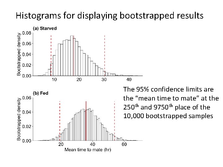
Histograms for displaying bootstrapped results The 95% confidence limits are the “mean time to mate” at the 250 th and 9750 th place of the 10, 000 bootstrapped samples
- Slides: 30