Nonparametric Statistical Methods Svetlana Stoyanchev Luke Schordine Li

Nonparametric Statistical Methods Svetlana Stoyanchev Luke Schordine Li Ouyang Valencia Joseph Minghui Lu Rachel Merrill Kleva Costa Michael Johnes Jane Cerise Statistics and Data Analysis Chapter 14 December 13, 2007 1

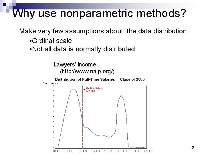
Why use nonparametric methods? Make very few assumptions about the data distribution • Ordinal scale • Not all data is normally distributed Lawyers’ income (http: //www. nalp. org/) 3

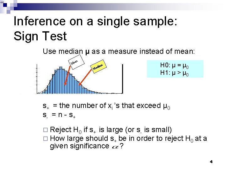
Inference on a single sample: Sign Test Use median μ as a measure instead of mean: an Me Me n dia H 0: μ = μ 0 H 1: μ > μ 0 s+ = the number of xi ’s that exceed μ 0 s- = n - s+ ¨ Reject H 0 if s+ is large (or s- is small) ¨ How large should s+ be in order to reject H 0 at a given significance ? 4

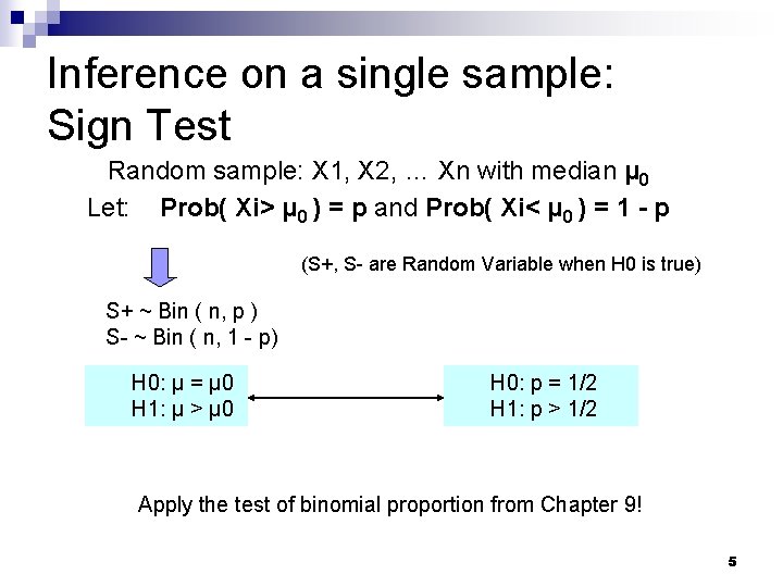
Inference on a single sample: Sign Test Random sample: X 1, X 2, … Xn with median μ 0 Let: Prob( Xi> μ 0 ) = p and Prob( Xi< μ 0 ) = 1 - p (S+, S- are Random Variable when H 0 is true) S+ ~ Bin ( n, p ) S- ~ Bin ( n, 1 - p) H 0: μ = μ 0 H 1: μ > μ 0 H 0: p = 1/2 H 1: p > 1/2 Apply the test of binomial proportion from Chapter 9! 5

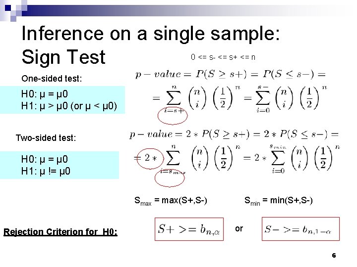
Inference on a single sample: Sign Test 0 <= s- <= s+ <= n One-sided test: H 0: μ = μ 0 H 1: μ > μ 0 (or μ < μ 0) Two-sided test: H 0: μ = μ 0 H 1: μ != μ 0 Smax = max(S+, S-) Rejection Criterion for H 0: Smin = min(S+, S-) or 6

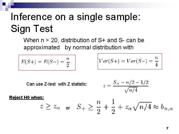
Inference on a single sample: Sign Test When n > 20, distribution of S+ and S- can be approximated by normal distribution with Can use Z-test with Z statistic: Reject H 0 when: or 7

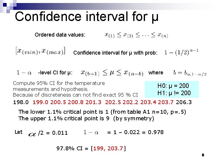
Confidence interval for μ Ordered data values: Confidence interval for μ with prob: -level CI for μ: where Compute 95% CI for the temperature measurements and hypothesis. Because of discreteness can not find exact 95 % CI H 0: μ = 200 H 1: μ != 200 198. 0 199. 0 200. 5 200. 8 201. 3 202. 5 202. 2 203. 4 203. 7 206. 3 The lower 1. 1% critical point is 1 (from table A 1 n=10, p=. 5) The upper 1. 1% critical point is 9 (by symmetry) Let /2 = 0. 011 = 1 – 0. 022 = 0. 978 97. 8% CI = [199, 203. 7] 8

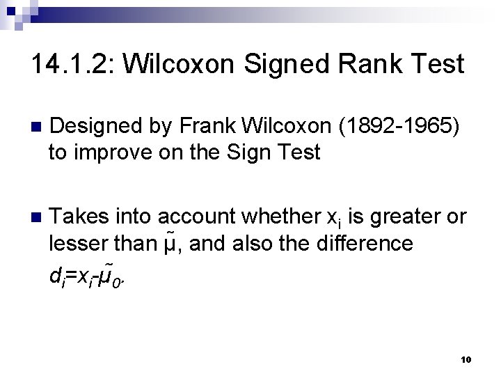
14. 1. 2: Wilcoxon Signed Rank Test n Designed by Frank Wilcoxon (1892 -1965) to improve on the Sign Test n Takes into account whether xi is greater or lesser than µ , and also the difference di=xi-µ 0. 10

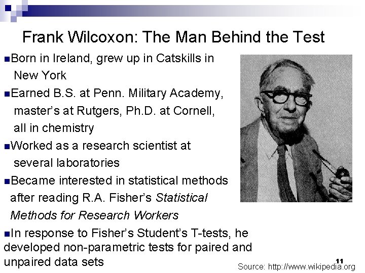
Frank Wilcoxon: The Man Behind the Test n. Born in Ireland, grew up in Catskills in New York n. Earned B. S. at Penn. Military Academy, master’s at Rutgers, Ph. D. at Cornell, all in chemistry n. Worked as a research scientist at several laboratories n. Became interested in statistical methods after reading R. A. Fisher’s Statistical Methods for Research Workers n. In response to Fisher’s Student’s T-tests, he developed non-parametric tests for paired and 11 unpaired data sets Source: http: //www. wikipedia. org

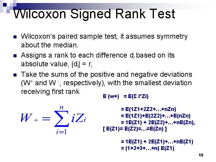
Wilcoxon Signed Rank Test n n n Wilcoxon’s paired sample test, it assumes symmetry about the median. Assigns a rank to each difference di based on its absolute value, |di| = ri Take the sums of the positive and negative deviations (W+ and W -, respectively), with the smallest deviation receiving first rank E (w+) = E(Σ i*Zi) = E(1 Z 1+2 Z 2+…+n. Zn) = E(1 Z 1)+E(2 Z 2)+…+E(n. Zn) = 1 E(Z 1) + 2 E(Z 2)+…+n. E(Zn), [ E(Z 1)= E(Z 2)=…=E(Zn) ] = 1 E(Z 1) + 2 E(Z 1)+…+n. E(Z 1) = (1+2+3+…+n) E(Z 1) 12

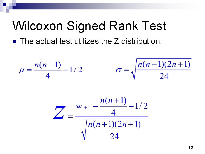
Wilcoxon Signed Rank Test n The actual test utilizes the Z distribution: 13

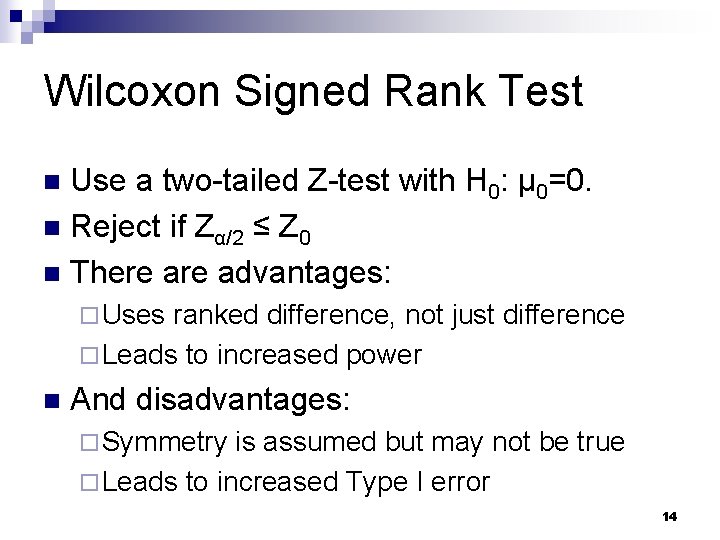
Wilcoxon Signed Rank Test Use a two-tailed Z-test with H 0: μ 0=0. n Reject if Zα/2 ≤ Z 0 n There advantages: n ¨ Uses ranked difference, not just difference ¨ Leads to increased power n And disadvantages: ¨ Symmetry is assumed but may not be true ¨ Leads to increased Type I error 14

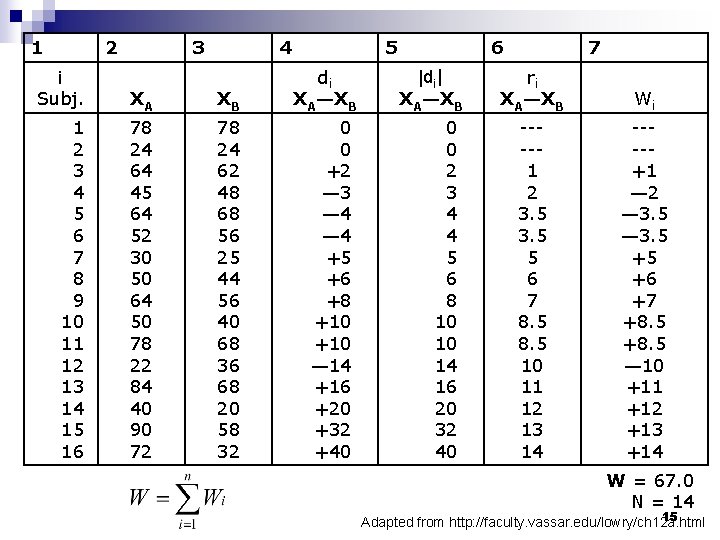
1 2 i Subj. 1 2 3 4 5 6 7 8 9 10 11 12 13 14 15 16 3 4 XA XB 78 24 64 45 64 52 30 50 64 50 78 22 84 40 90 72 78 24 62 48 68 56 25 44 56 40 68 36 68 20 58 32 5 6 |di| XA—XB di XA—XB 0 0 +2 — 3 — 4 +5 +6 +8 +10 — 14 +16 +20 +32 +40 0 0 2 3 4 4 5 6 8 10 14 16 20 32 40 7 ri XA—XB Wi ----1 2 3. 5 5 6 7 8. 5 10 11 12 13 14 ----+1 — 2 — 3. 5 +5 +6 +7 +8. 5 — 10 +11 +12 +13 +14 W = 67. 0 TN = 14 15 Adapted from http: //faculty. vassar. edu/lowry/ch 12 a. html

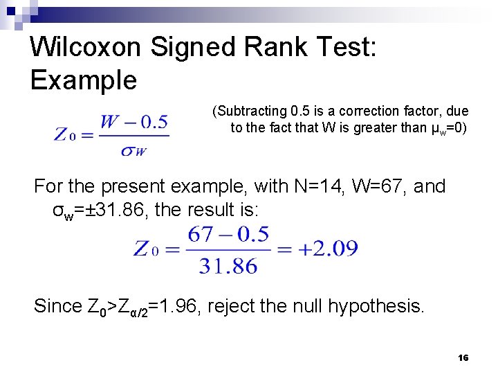
Wilcoxon Signed Rank Test: Example (Subtracting 0. 5 is a correction factor, due to the fact that W is greater than μw=0) For the present example, with N=14, W=67, and σw=± 31. 86, the result is: Since Z 0>Zα/2=1. 96, reject the null hypothesis. 16

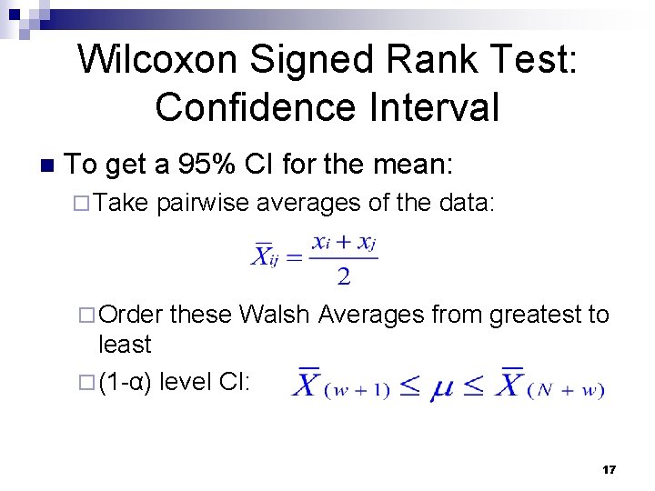
Wilcoxon Signed Rank Test: Confidence Interval n To get a 95% CI for the mean: ¨ Take pairwise averages of the data: ¨ Order these Walsh Averages from greatest to least ¨ (1 -α) level CI: 17

14. 2 Inferences for Two Independent Samples By -Li Ouyang 18

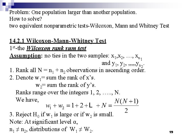
Problem: One population larger than another population. How to solve? two equivalent nonparametric tests-Wilcoxon, Mann and Whitney Test 14. 2. 1 Wilcoxon-Mann-Whitney Test 1 st-the Wilcoxon rank sum test Assumption: no ties in the two samples: x 1, x 2, …, xn 1 and y 1, y 2, , , yn 2. 1. Rank all N = n 1 + n 2 observations in ascending order. 2. Denote w 1= sum the rank of x’s. w 2= sum the rank of y’s. Ranks range over the integers 1, 2, …. . , N. We have, 3. Reject H 0 if w 1 is large or if w 2 is small. Note: At significant level α, n 1 ≠ n 2, distributions of W 1 ≠ W 2. 19

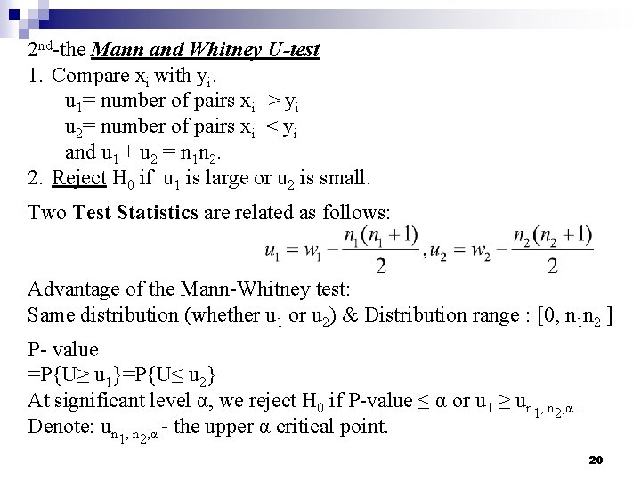
2 nd-the Mann and Whitney U-test 1. Compare xi with yi. u 1= number of pairs xi > yi u 2= number of pairs xi < yi and u 1 + u 2 = n 1 n 2. 2. Reject H 0 if u 1 is large or u 2 is small. Two Test Statistics are related as follows: Advantage of the Mann-Whitney test: Same distribution (whether u 1 or u 2) & Distribution range : [0, n 1 n 2 ] P- value =P{U≥ u 1}=P{U≤ u 2} At significant level α, we reject H 0 if P-value ≤ α or u 1 ≥ un 1, n 2, α. Denote: un 1, n 2, α - the upper α critical point. 20

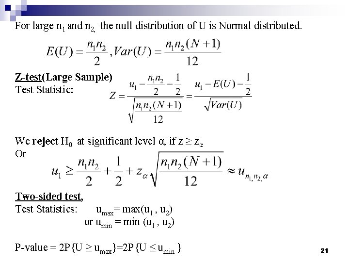
For large n 1 and n 2, the null distribution of U is Normal distributed. Z-test(Large Sample) Test Statistic: We reject H 0 at significant level α, if z ≥ zα Or Two-sided test, Test Statistics: umax= max(u 1 , u 2) or umin = min (u 1 , u 2) P-value = 2 P{U ≥ umax}=2 P{U ≤ umin } 21

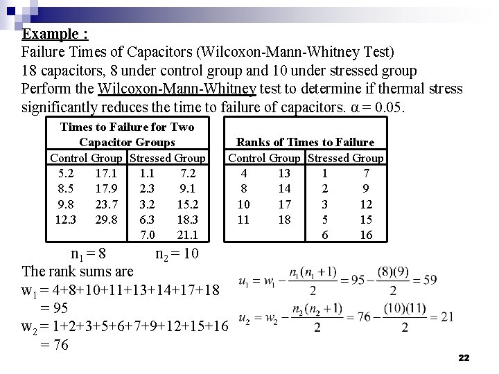
Example : Failure Times of Capacitors (Wilcoxon-Mann-Whitney Test) 18 capacitors, 8 under control group and 10 under stressed group Perform the Wilcoxon-Mann-Whitney test to determine if thermal stress significantly reduces the time to failure of capacitors. α = 0. 05. Times to Failure for Two Capacitor Groups Control Group Stressed Group 5. 2 17. 1 1. 1 7. 2 8. 5 17. 9 2. 3 9. 1 9. 8 23. 7 3. 2 15. 2 12. 3 29. 8 6. 3 18. 3 7. 0 21. 1 Ranks of Times to Failure Control Group Stressed Group 4 13 1 7 8 14 2 9 10 17 3 12 11 18 5 15 6 16 n 1 = 8 n 2 = 10 The rank sums are w 1 = 4+8+10+11+13+14+17+18 = 95 w 2 = 1+2+3+5+6+7+9+12+15+16 = 76 22

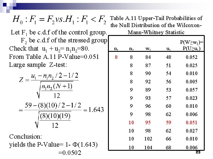
Table A. 11 Upper-Tail Probabilities of the Null Distribution of the Wilcoxon. Mann-Whitney Statistic Let F 1 be c. d. f of the control group. F 2 be c. d. f of the stressed group. Check that u 1 + u 2= n 1 n 2=80. From Table A. 11 P-Value=0. 051 Large sample Z-test: Conclusion: yields the P-Value= 1 - Ф(1. 643) =0. 0502 n 1 n 2 w 1 u 1 P(W≥w 1)= P(U≥u 1) 8 8 84 48 0. 052 8 87 51 0. 025 8 90 54 0. 010 8 92 56 0. 005 9 89 53 0. 057 9 93 57 0. 023 9 96 60 0. 010 9 98 62 0. 006 10 95 59 0. 051 10 98 62 0. 027 10 102 66 0. 010 10 104 68 0. 006 23

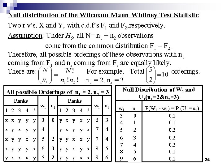
Null distribution of the Wilcoxon-Mann-Whitney Test Statistic Two r. v’s, X and Y, with c. d. f’s F 1 and F 2, respectively. Assumption: Under H 0, all N= n 1 + n 2 observations come from the common distribution F 1 = F 2. Therefore, all possible orderings of these observations with n 1 coming from F 1 and n 2 coming from F 2 are equally likely. There are: For example, Total orderings. n 1 = 2, n 2 = 3. All possible Orderings of n 1 = 2, n 2 = 3 Ranks 1 2 3 4 5 w 1 u 1 x x y y y 3 0 y x y 6 3 x y y 4 1 y x y y x 7 4 x y y x y 5 2 y y x x y 7 4 x y y y x 6 3 y y x 8 5 y x x x y 5 2 y y y x x 9 6 Null Distribution of W 1 and U 1(n 1=2&n 2=3) w 1 3 4 5 6 7 8 9 u 1 0 1 2 3 4 5 6 P(W 1 - w 1) = P (U 1 =u 1) 0. 1 0. 2 0. 1 24

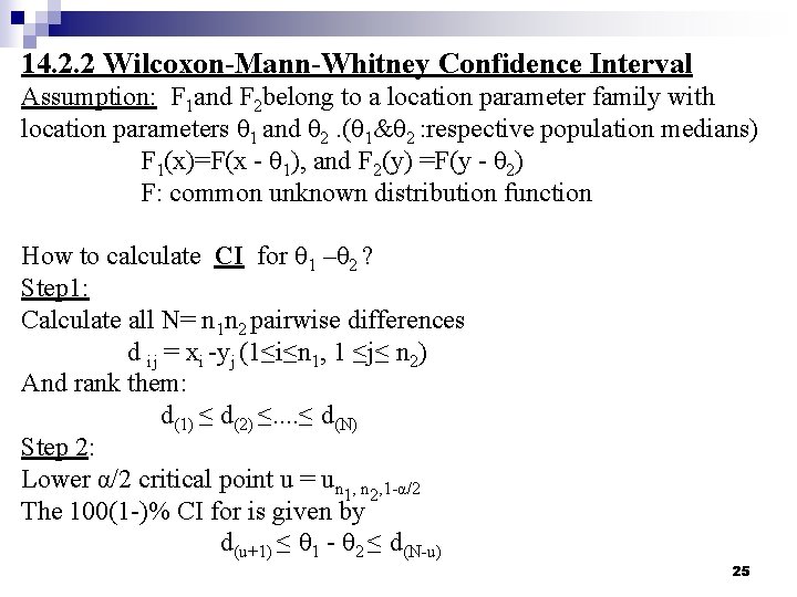
14. 2. 2 Wilcoxon-Mann-Whitney Confidence Interval Assumption: F 1 and F 2 belong to a location parameter family with location parameters θ 1 and θ 2. (θ 1&θ 2 : respective population medians) F 1(x)=F(x - θ 1), and F 2(y) =F(y - θ 2) F: common unknown distribution function How to calculate CI for θ 1 –θ 2 ? Step 1: Calculate all N= n 1 n 2 pairwise differences d ij = xi -yj (1≤i≤n 1, 1 ≤j≤ n 2) And rank them: d(1) ≤ d(2) ≤. . ≤ d(N) Step 2: Lower α/2 critical point u = un 1, n 2, 1 -α/2 The 100(1 -)% CI for is given by d(u+1) ≤ θ 1 - θ 2 ≤ d(N-u) 25

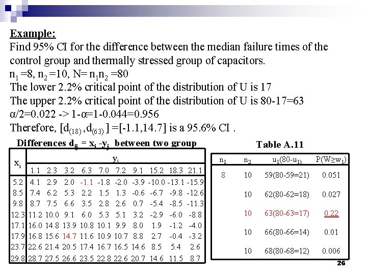
Example: Find 95% CI for the difference between the median failure times of the control group and thermally stressed group of capacitors. n 1 =8, n 2 =10, N= n 1 n 2 =80 The lower 2. 2% critical point of the distribution of U is 17 The upper 2. 2% critical point of the distribution of U is 80 -17=63 α/2=0. 022 -> 1 -α=1 -0. 044=0. 956 Therefore, [d(18) , d(63) ] =[-1. 1, 14. 7] is a 95. 6% CI. Differences dij = xi -yj between two group xi 5. 2 8. 5 9. 8 12. 3 17. 1 17. 9 23. 7 29. 8 yi 1. 1 4. 1 7. 4 8. 7 11. 2 16. 0 16. 8 22. 6 28. 7 2. 3 2. 9 6. 2 7. 5 10. 0 14. 8 15. 6 21. 4 27. 5 3. 2 2. 0 5. 3 6. 6 9. 1 13. 9 14. 7 20. 5 26. 6 6. 3 -1. 1 2. 2 3. 5 6. 0 10. 8 11. 6 17. 4 23. 5 7. 0 -1. 8 1. 5 2. 8 5. 3 10. 1 10. 9 16. 7 22. 8 7. 2 -2. 0 1. 3 2. 6 5. 1 9. 9 10. 7 16. 5 22. 6 9. 1 -3. 9 -0. 6 0. 7 3. 2 8. 0 8. 8 14. 6 20. 7 15. 2 18. 3 21. 1 -10. 0 -13. 1 -15. 9 -6. 7 -9. 8 -12. 6 -5. 4 -8. 5 -11. 3 -2. 9 -6. 0 -8. 8 1. 9 -1. 2 -4. 0 2. 7 -0. 4 -3. 2 8. 5 5. 4 2. 6 14. 6 11. 5 8. 7 Table A. 11 n 1 n 2 u 1(80 -u 1) P(W≥w 1) 8 10 59(80 -59=21) 0. 051 10 62(80 -62=18) 0. 027 10 63(80 -63=17) 0. 22 10 66(80 -66=14) 0. 01 10 68(80 -68=12) 0. 006 26

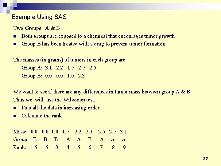
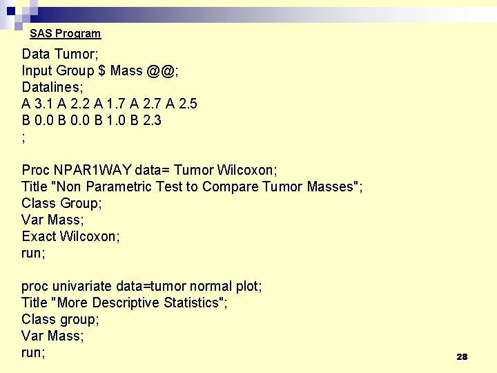
Example Using SAS Two Groups A & B n Both groups are exposed to a chemical that encourages tumor growth n Group B has been treated with a drug to prevent tumor formation The masses (in grams) of tumors in each group are Group A: 3. 1 2. 2 1. 7 2. 5 Group B: 0. 0 1. 0 2. 3 We want to see if there any differences in tumor mass between group A & B. Thus we will use the Wilcoxon test. n Puts all the data in increasing order n Calculate the rank Mass: 0. 0 1. 0 1. 7 2. 2 2. 3 2. 5 2. 7 3. 1 Group: B B B A A A Rank: 1. 5 3 4 5 6 7 8 9 27

SAS Program Data Tumor; Input Group $ Mass @@; Datalines; A 3. 1 A 2. 2 A 1. 7 A 2. 5 B 0. 0 B 1. 0 B 2. 3 ; Proc NPAR 1 WAY data= Tumor Wilcoxon; Title "Non Parametric Test to Compare Tumor Masses"; Class Group; Var Mass; Exact Wilcoxon; run; proc univariate data=tumor normal plot; Title "More Descriptive Statistics"; Class group; Var Mass; run; 28

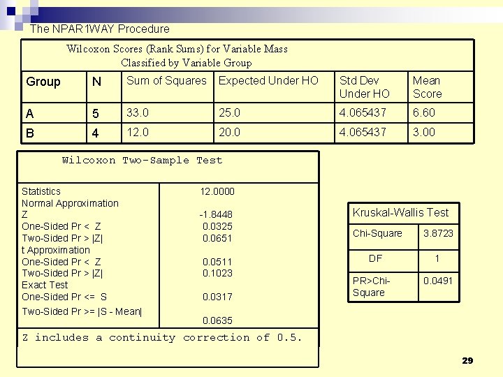
The NPAR 1 WAY Procedure Wilcoxon Scores (Rank Sums) for Variable Mass Classified by Variable Group N Sum of Squares Expected Under HO Std Dev Under HO Mean Score A 5 33. 0 25. 0 4. 065437 6. 60 B 4 12. 0 20. 0 4. 065437 3. 00 Wilcoxon Two-Sample Test Statistics Normal Approximation Z One-Sided Pr < Z Two-Sided Pr > |Z| t Approximation One-Sided Pr < Z Two-Sided Pr > |Z| Exact Test One-Sided Pr <= S Two-Sided Pr >= |S - Mean| 12. 0000 -1. 8448 0. 0325 0. 0651 Kruskal-Wallis Test Chi-Square 3. 8723 0. 0511 0. 1023 0. 0317 0. 0635 DF 1 PR>Chi. Square 0. 0491 Z includes a continuity correction of 0. 5. 29

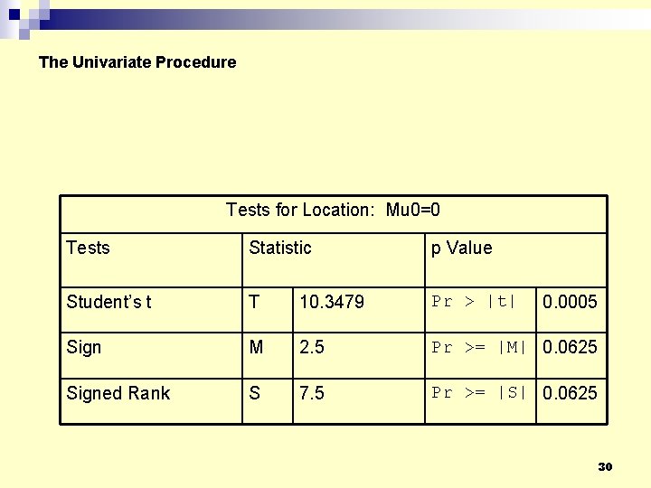
The Univariate Procedure Tests for Location: Mu 0=0 Tests Statistic p Value Student’s t T 10. 3479 Pr > |t| Sign M 2. 5 Pr >= |M| 0. 0625 Signed Rank S 7. 5 Pr >= |S| 0. 0625 0. 0005 30

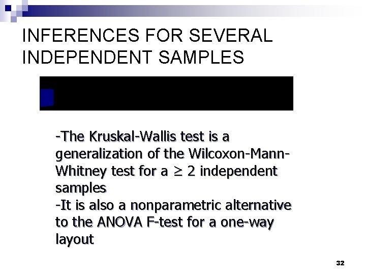
INFERENCES FOR SEVERAL INDEPENDENT SAMPLES -The Kruskal-Wallis test is a generalization of the Wilcoxon-Mann. Whitney test for a ≥ 2 independent samples -It is also a nonparametric alternative to the ANOVA F-test for a one-way layout 32

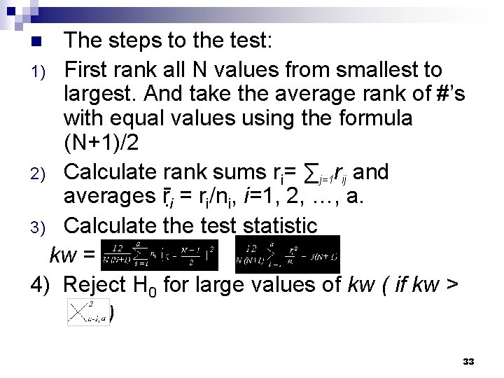
The steps to the test: 1) First rank all N values from smallest to largest. And take the average rank of #’s with equal values using the formula (N+1)/2 2) Calculate rank sums ri= ∑j=1 rij and averages ṝi = ri/ni, i=1, 2, …, a. 3) Calculate the test statistic kw = = 4) Reject H 0 for large values of kw ( if kw > ) n 33

The Pedagogy Problem Consider Example 14. 9 on page 581 of the text, in which four methods of teaching the concept of percentage to sixth graders are compared. There are 28 classes, 7 using each method: the Case Method, the Formula Method, the Equation Method, and the Unitary Analysis Method. 34

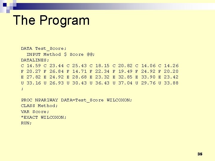
The Program DATA Test_Score; INPUT Method $ Score @@; DATALINES; C 14. 59 C 23. 44 C 25. 43 C 18. 15 F 20. 27 F 26. 84 F 14. 71 F 22. 34 E 27. 82 E 24. 92 E 28. 68 E 23. 32 U 33. 16 U 26. 93 U 30. 43 U 36. 43 ; C F E U 20. 82 19. 49 32. 85 37. 04 C F E U 14. 06 24. 92 33. 90 29. 76 C F E U 14. 26 20. 20 23. 42 33. 88 PROC NPAR 1 WAY DATA=Test_Score WILCOXON; CLASS Method; VAR Score; *EXACT WILCOXON; RUN; 35

A Note About the Program You might have noticed the asterisk in the program line: *EXACT WILCOXON The asterisk turns the line into a comment. Otherwise, SAS attempts to find an exact pvalue for the test, and it can take a very long time. Otherwise, this command would be highly recommended. We’ll settle for a quicker approximation. 36

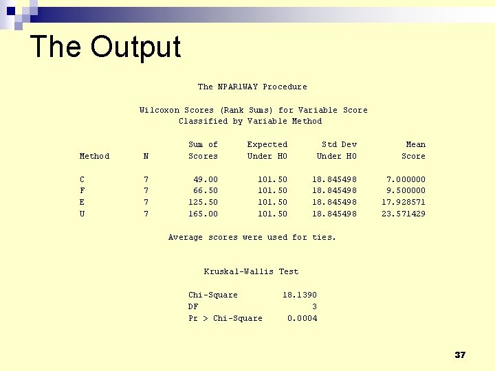
The Output The NPAR 1 WAY Procedure Wilcoxon Scores (Rank Sums) for Variable Score Classified by Variable Method N Sum of Scores C F E U 7 7 49. 00 66. 50 125. 50 165. 00 Expected Under H 0 Std Dev Under H 0 Mean Score 101. 50 18. 845498 7. 000000 9. 500000 17. 928571 23. 571429 Average scores were used for ties. Kruskal-Wallis Test Chi-Square DF Pr > Chi-Square 18. 1390 3 0. 0004 37

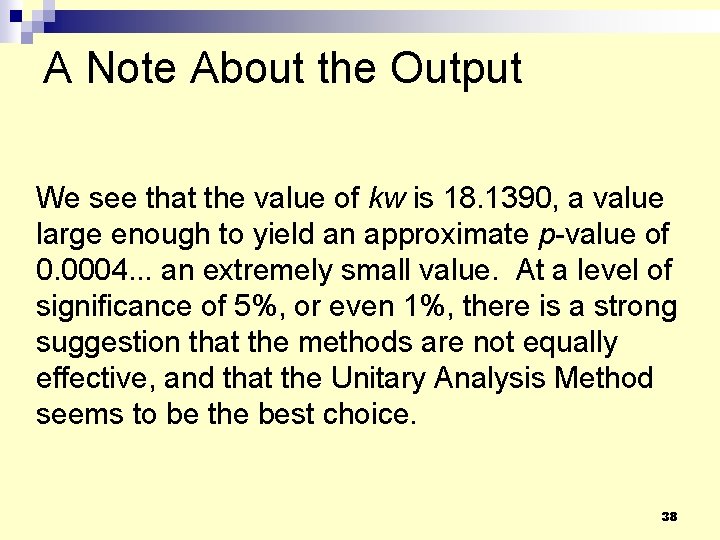
A Note About the Output We see that the value of kw is 18. 1390, a value large enough to yield an approximate p-value of 0. 0004. . . an extremely small value. At a level of significance of 5%, or even 1%, there is a strong suggestion that the methods are not equally effective, and that the Unitary Analysis Method seems to be the best choice. 38

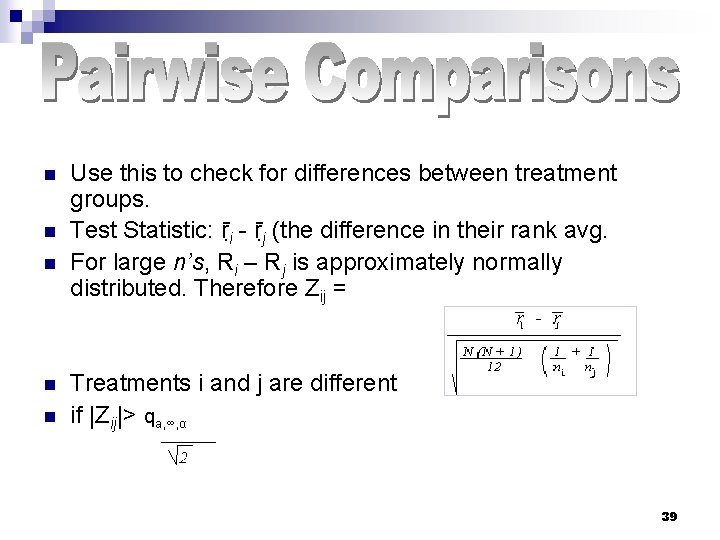
n n n Use this to check for differences between treatment groups. Test Statistic: ṝi - ṝj (the difference in their rank avg. For large n’s, Ri – Rj is approximately normally distributed. Therefore Zij = Treatments i and j are different if |Zij|> qa, ∞, α 39

INFERENCES FOR SEVERAL MATCHED SAMPLES n n n The Friedman Test is a generalization of the sign test for a ≥ 2 matched samples It is also a nonparametric alternative to the ANOVA FTest for a randomized block design Since this is use for a block design, rankings are done within each individual group. The steps for the test: Rank observations from a treatments separately within each block. Where needed take the average of equal ranking values using (N+ 2) /2. 40

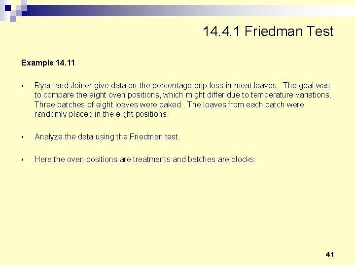
14. 4. 1 Friedman Test Example 14. 11 § Ryan and Joiner give data on the percentage drip loss in meat loaves. The goal was to compare the eight oven positions, which might differ due to temperature variations. Three batches of eight loaves were baked. The loaves from each batch were randomly placed in the eight positions. § Analyze the data using the Friedman test. § Here the oven positions are treatments and batches are blocks. 41

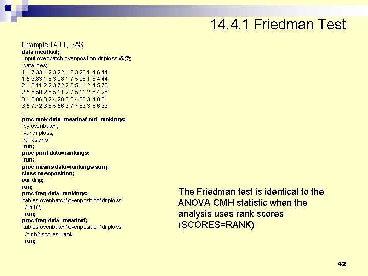
14. 4. 1 Friedman Test Example 14. 11, SAS data meatloaf; input ovenbatch ovenposition driploss @@; datalines; 1 1 7. 33 1 2 3. 22 1 3 3. 28 1 4 6. 44 1 5 3. 83 1 6 3. 28 1 7 5. 06 1 8 4. 44 2 1 8. 11 2 2 3. 72 2 3 5. 11 2 4 5. 78 2 5 6. 50 2 6 5. 11 2 7 5. 11 2 8 4. 28 3 1 8. 06 3 2 4. 28 3 3 4. 56 3 4 8. 61 3 5 7. 72 3 6 5. 56 3 7 7. 83 3 8 6. 33 ; proc rank data=meatloaf out=rankings; by ovenbatch; var driploss; ranks drip; run; proc print data=rankings; run; proc means data=rankings sum; class ovenposition; var drip; run; proc freq data=rankings; tables ovenbatch*ovenposition*driploss /cmh 2; run; proc freq data=meatloaf; tables ovenbatch*ovenposition*driploss /cmh 2 scores=rank; run; The Friedman test is identical to the ANOVA CMH statistic when the analysis uses rank scores (SCORES=RANK) 42

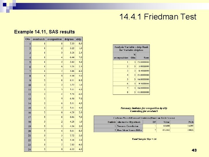
14. 4. 1 Friedman Test Example 14. 11, SAS results 43

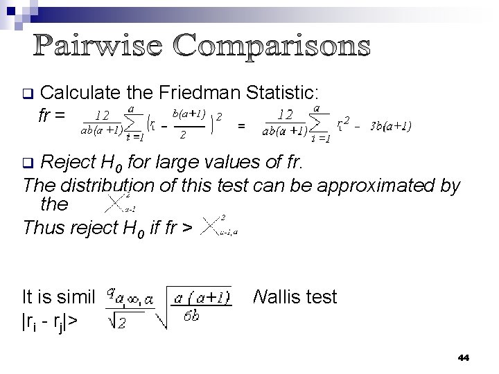
Calculate the Friedman Statistic: fr = = q Reject H 0 for large values of fr. The distribution of this test can be approximated by the Thus reject H 0 if fr > q It is similar to the Kruskal- Wallis test |ri - rj|> 44

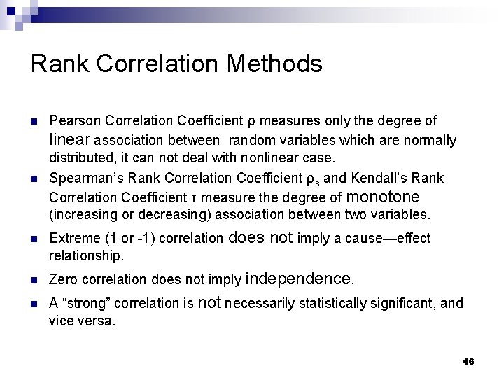
Rank Correlation Methods n n n Pearson Correlation Coefficient ρ measures only the degree of linear association between random variables which are normally distributed, it can not deal with nonlinear case. Spearman’s Rank Correlation Coefficient ρs and Kendall’s Rank Correlation Coefficient τ measure the degree of monotone (increasing or decreasing) association between two variables. Extreme (1 or -1) correlation does not imply a cause—effect relationship. Zero correlation does not imply independence. A “strong” correlation is not necessarily statistically significant, and vice versa. 46

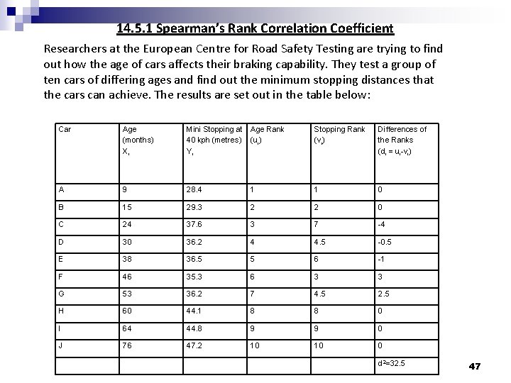
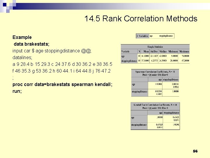
14. 5. 1 Spearman’s Rank Correlation Coefficient Researchers at the European Centre for Road Safety Testing are trying to find out how the age of cars affects their braking capability. They test a group of ten cars of differing ages and find out the minimum stopping distances that the cars can achieve. The results are set out in the table below: Car Age (months) Xi Mini Stopping at Age Rank 40 kph (metres) (ui) Yi Stopping Rank (vi) Differences of the Ranks (di = ui-vi) A 9 28. 4 1 1 0 B 15 29. 3 2 2 0 C 24 37. 6 3 7 -4 D 30 36. 2 4 4. 5 -0. 5 E 38 36. 5 5 6 -1 F 46 35. 3 6 3 3 G 53 36. 2 7 4. 5 2. 5 H 60 44. 1 8 8 0 I 64 44. 8 9 9 0 J 76 47. 2 10 10 0 d 2=32. 5 47

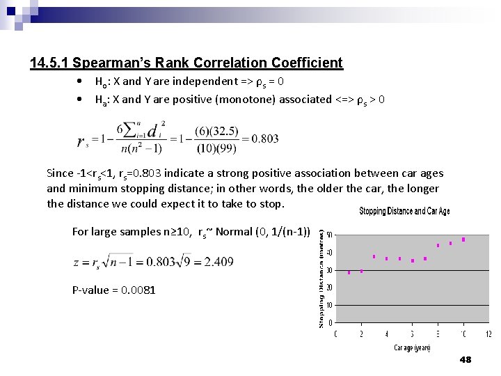
14. 5. 1 Spearman’s Rank Correlation Coefficient • Ho: X and Y are independent => ρs = 0 • Ha: X and Y are positive (monotone) associated <=> ρs > 0 Since -1<rs<1, rs=0. 803 indicate a strong positive association between car ages and minimum stopping distance; in other words, the older the car, the longer the distance we could expect it to take to stop. For large samples n≥ 10, rs~ Normal (0, 1/(n-1)) P-value = 0. 0081 48

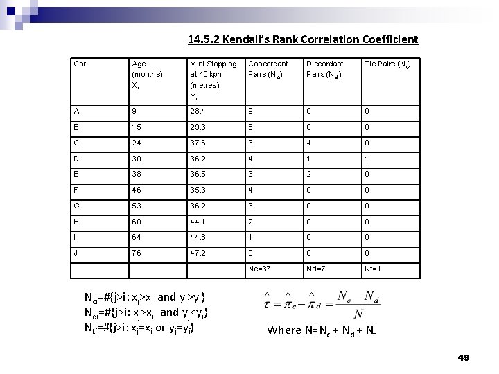
14. 5. 2 Kendall’s Rank Correlation Coefficient Car Age (months) Xi Mini Stopping at 40 kph (metres) Yi Concordant Pairs (Nci) Discordant Pairs (Ndi) Tie Pairs (Nti) A 9 28. 4 9 0 0 B 15 29. 3 8 0 0 C 24 37. 6 3 4 0 D 30 36. 2 4 1 1 E 38 36. 5 3 2 0 F 46 35. 3 4 0 0 G 53 36. 2 3 0 0 H 60 44. 1 2 0 0 I 64 44. 8 1 0 0 J 76 47. 2 0 0 0 Nc=37 Nd=7 Nt=1 Nci=#{j>i: xj>xi and yj>yi} Ndi=#{j>i: xj>xi and yj<yi} Nti=#{j>i: xj=xi or yj=yi} Where N=Nc + Nd + Nt 49

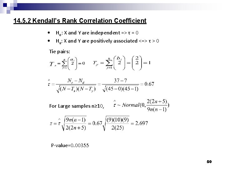
14. 5. 2 Kendall’s Rank Correlation Coefficient • Ho: X and Y are independent => τ = 0 • Ha: X and Y are positively associated <=> τ > 0 Tie pairs: For Large samples n≥ 10, P-value=0. 00355 50

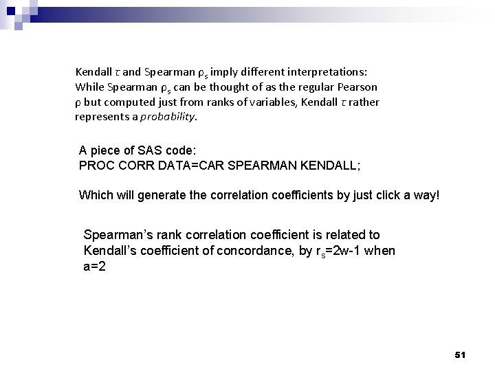
Kendall τ and Spearman ρs imply different interpretations: While Spearman ρs can be thought of as the regular Pearson ρ but computed just from ranks of variables, Kendall τ rather represents a probability. A piece of SAS code: PROC CORR DATA=CAR SPEARMAN KENDALL; Which will generate the correlation coefficients by just click a way! Spearman’s rank correlation coefficient is related to Kendall’s coefficient of concordance, by rs=2 w-1 when a=2 51

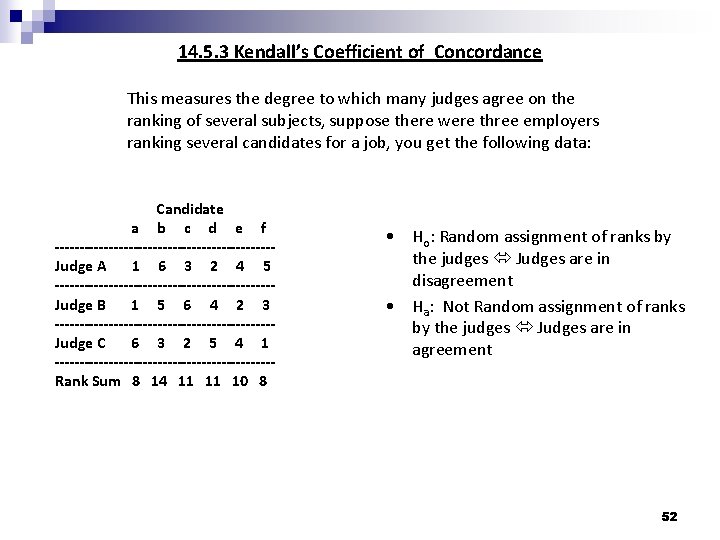
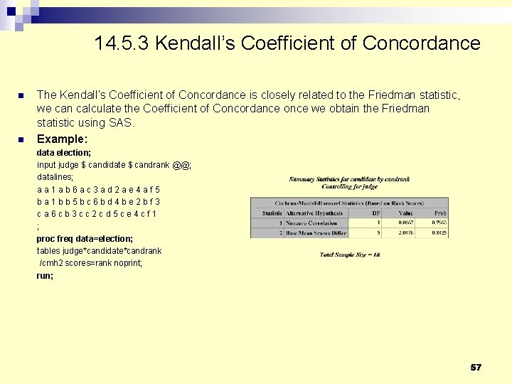
14. 5. 3 Kendall’s Coefficient of Concordance This measures the degree to which many judges agree on the ranking of several subjects, suppose there were three employers ranking several candidates for a job, you get the following data: Candidate a b c d e f ----------------------Judge A 1 6 3 2 4 5 ----------------------Judge B 1 5 6 4 2 3 ----------------------Judge C 6 3 2 5 4 1 ----------------------Rank Sum 8 14 11 11 10 8 • Ho: Random assignment of ranks by the judges Judges are in disagreement • Ha: Not Random assignment of ranks by the judges Judges are in agreement 52

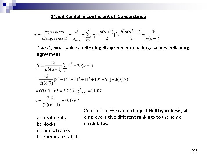
14. 5. 3 Kendall’s Coefficient of Concordance 0≤w≤ 1, small values indicating disagreement and large values indicating agreement a: treatments b: blocks ri: sum of ranks fr: Friedman statistic Conclusion: We can not reject Null hypothesis, all employers give different rankings to the same candidates. 53

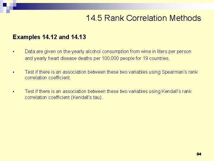
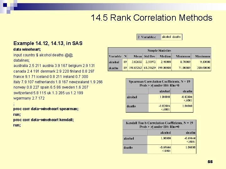
14. 5 Rank Correlation Methods Examples 14. 12 and 14. 13 § Data are given on the yearly alcohol consumption from wine in liters person and yearly heart disease deaths per 100, 000 people for 19 countries. § Test if there is an association between these two variables using Spearman’s rank correlation coefficient. § Test if there is an association between these two variables using Kendall’s rank correlation coefficient (Kendall’s tau). 54

14. 5 Rank Correlation Methods Example 14. 12, 14. 13, in SAS data wineheart; input country $ alcohol deaths @@; datalines; australia 2. 5 211 austria 3. 9 167 belgium 2. 9 131 canada 2. 4 191 denmark 2. 9 220 finland 0. 8 297 france 9. 1 71 iceland 0. 8 211 ireland 0. 7 300 italy 7. 9 107 netherlands 1. 8 167 newzealand 1. 9 266 norway 0. 8 227 spain 6. 5 86 sweden 1. 6 207 switzerland 5. 8 115 uk 1. 3 285 us 1. 2 199 wgermany 2. 7 172 ; proc corr data=wineheart spearman; run; proc corr data=wineheart kendall; run; 55

14. 5 Rank Correlation Methods Example data brakestats; input car $ age stoppingdistance @@; datalines; a 9 28. 4 b 15 29. 3 c 24 37. 6 d 30 36. 2 e 38 36. 5 f 46 35. 3 g 53 36. 2 h 60 44. 1 i 64 44. 8 j 76 47. 2 ; proc corr data=brakestats spearman kendall; run; 56

14. 5. 3 Kendall’s Coefficient of Concordance n n The Kendall’s Coefficient of Concordance is closely related to the Friedman statistic, we can calculate the Coefficient of Concordance once we obtain the Friedman statistic using SAS. Example: data election; input judge $ candidate $ candrank @@; datalines; a a 1 a b 6 a c 3 a d 2 a e 4 a f 5 b a 1 b b 5 b c 6 b d 4 b e 2 b f 3 c a 6 c b 3 c c 2 c d 5 c e 4 c f 1 ; proc freq data=election; tables judge*candidate*candrank /cmh 2 scores=rank noprint; run; 57

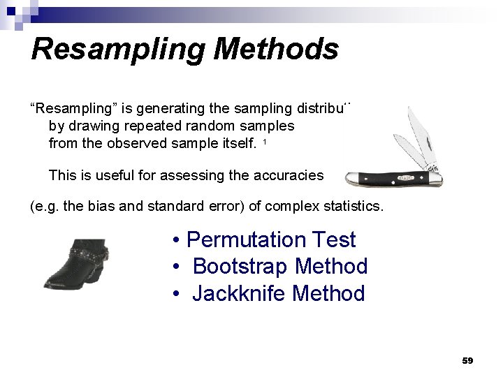
Resampling Methods “Resampling” is generating the sampling distribution by drawing repeated random samples from the observed sample itself. 1 This is useful for assessing the accuracies (e. g. the bias and standard error) of complex statistics. • Permutation Test • Bootstrap Method • Jackknife Method 59

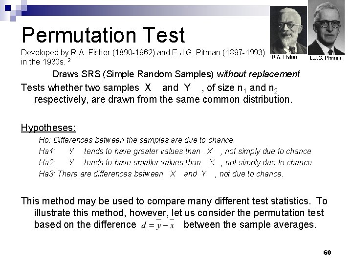
Permutation Test Developed by R. A. Fisher (1890 -1962) and E. J. G. Pitman (1897 -1993) in the 1930 s. 2 Draws SRS (Simple Random Samples) without replacement Tests whether two samples X and Y , of size n 1 and n 2 respectively, are drawn from the same common distribution. Hypotheses: Ho: Differences between the samples are due to chance. Ha 1: Y tends to have greater values than X , not simply due to chance Ha 2: Y tends to have smaller values than X , not simply due to chance Ha 3: There are differences between X and Y , not due to chance. This method may be used to compare many different test statistics. To illustrate this method, however, let us consider the permutation test based on the difference between the sample averages. 60

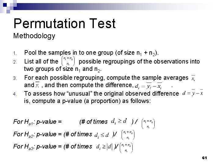
Permutation Test Methodology 1. 2. 3. 4. Pool the samples in to one group (of size n 1 + n 2). List all of the possible regroupings of the observations into two groups of size n 1 and n 2. For each possible regrouping, compute the sample averages and , and then compute the difference, . To assess how “unusual” the original observed difference is, compute a p-value (a proportion) as follows: For Ha 1: p-value = (# of times )/ For Ha 2: p-value = (# of times )/ For Ha 3: p-value = (# of times )/ 61

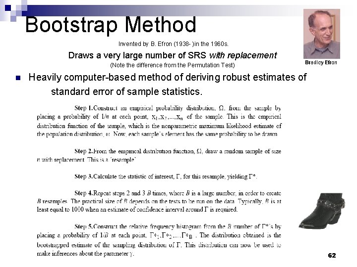
Bootstrap Method Invented by B. Efron (1938 - )in the 1960 s. Draws a very large number of SRS with replacement (Note the difference from the Permutation Test) n Heavily computer-based method of deriving robust estimates of standard error of sample statistics. 62

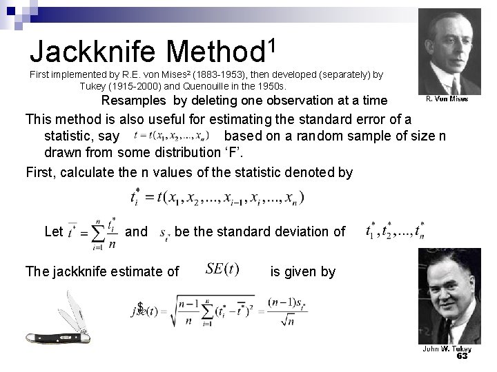
Jackknife Method 1 First implemented by R. E. von Mises 2 (1883 -1953), then developed (separately) by Tukey (1915 -2000) and Quenouille in the 1950 s. Resamples by deleting one observation at a time This method is also useful for estimating the standard error of a statistic, say based on a random sample of size n drawn from some distribution ‘F’. First, calculate the n values of the statistic denoted by Let and be the standard deviation of The jackknife estimate of is given by 63

14. 6 Resampling Methods SAS can be used to perform permutation, bootstrap, and jackknife resampling. § § For the most part macros are required. These can be written and are also readily available on the web. § § PROC MULTTEST can be used to perform several tests incorporating permutation or bootstrap § In the following two examples, We use permutation and bootstrap resampling to obtain t-test p-value adjustment. 64

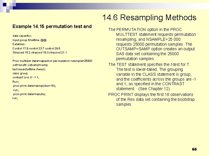
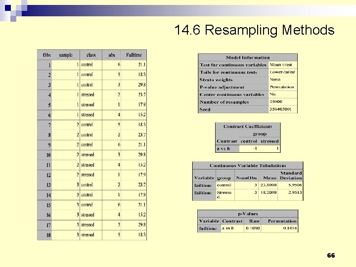
14. 6 Resampling Methods Example 14. 15 permutation test and data capacitor; Input group $ failtime @@; Datalines; Control 17. 9 control 23. 7 control 29. 8 Stressed 15. 2 stressed 18. 3 stressed 21. 1 ; Proc multtest data=capacitor permutation nsample=25000 out=results outsamp=samp; test mean(failtime /lower); class group; contrast 'a vs b' -1 1; Run; proc print data=samp(obs=18); run; proc print data=results; run; The PERMUTATION option in the PROC MULTTEST statement requests permutation resampling, and NSAMPLE=25 000 requests 25000 permutation samples. The OUTSAMP=SAMP option creates an output SAS data set containing the 25000 permutation samples. The TEST statement specifies the t-test for T. The test is lower-tailed. The grouping variable in the CLASS statement is group, and the coefficients across the groups are -1 and 1, as specified in the CONTRAST statement. (See Chapter 12) PROC PRINT displays the first 18 observations of the Res data set containing the bootstrap samples. 65

14. 6 Resampling Methods 66

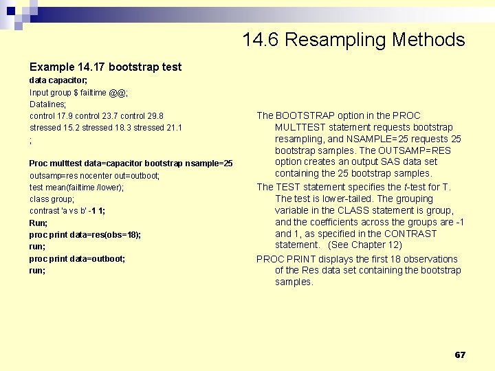
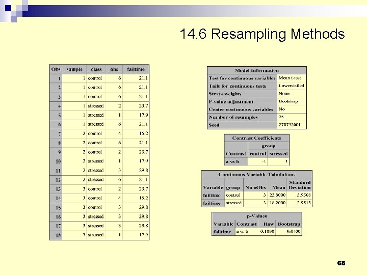
14. 6 Resampling Methods Example 14. 17 bootstrap test data capacitor; Input group $ failtime @@; Datalines; control 17. 9 control 23. 7 control 29. 8 stressed 15. 2 stressed 18. 3 stressed 21. 1 ; Proc multtest data=capacitor bootstrap nsample=25 outsamp=res nocenter out=outboot; test mean(failtime /lower); class group; contrast 'a vs b' -1 1; Run; proc print data=res(obs=18); run; proc print data=outboot; run; The BOOTSTRAP option in the PROC MULTTEST statement requests bootstrap resampling, and NSAMPLE=25 requests 25 bootstrap samples. The OUTSAMP=RES option creates an output SAS data set containing the 25 bootstrap samples. The TEST statement specifies the t-test for T. The test is lower-tailed. The grouping variable in the CLASS statement is group, and the coefficients across the groups are -1 and 1, as specified in the CONTRAST statement. (See Chapter 12) PROC PRINT displays the first 18 observations of the Res data set containing the bootstrap samples. 67

14. 6 Resampling Methods 68

Works Cited 1. 2. 3. Tamhane, Ajit and Dorothy Dunlop. Statistics and Data Analysis. Upper Saddle River, NJ. Prentice Hall, Inc. 2000. “Resampling (statistics)”. Wikipedia. <http: //en. wikipedia. org/wiki/Resampling_(statistics)>. 2007. “Ch. 14: Nonparametric Statistical Method” Group project, Wei Zhu, instructor. 2006. 69