Nonparametric Link Prediction in Dynamic Graphs Purnamrita Sarkar

Nonparametric Link Prediction in Dynamic Graphs Purnamrita Sarkar (UC Berkeley) Deepayan Chakrabarti (Facebook) Michael Jordan (UC Berkeley) 1

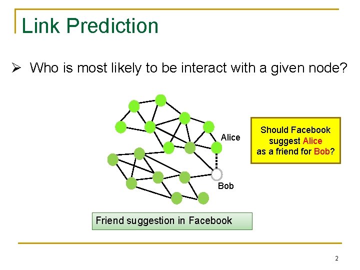
Link Prediction Ø Who is most likely to be interact with a given node? Alice Should Facebook suggest Alice as a friend for Bob? Bob Friend suggestion in Facebook 2

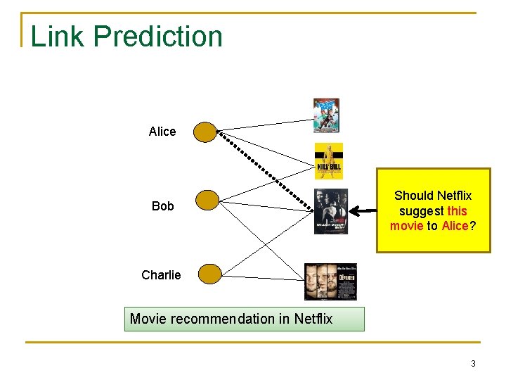
Link Prediction Alice Bob Should Netflix suggest this movie to Alice? Charlie Movie recommendation in Netflix 3

Link Prediction n Prediction using simple features q q q n degree of a node number of common neighbors last time a link appeared What if the graph is dynamic? 4

Related Work n Generative models q q q n Exp. family random graph models [Hanneke+/’ 06] Dynamics in latent space [Sarkar+/’ 05] Extension of mixed membership block models [Fu+/10] Other approaches q q Autoregressive models for links [Huang+/09] Extensions of static features [Tylenda+/09] 5

Goal n Link Prediction q q incorporating graph dynamics, requiring weak modeling assumptions, allowing fast predictions, and offering consistency guarantees. 6

Outline n n n Model Estimator Consistency Scalability Experiments 7

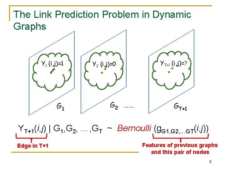
The Link Prediction Problem in Dynamic Graphs Y 1 (i, j)=1 G 1 Y 2 (i, j)=0 G 2 …… YT+1 (i, j)=? GT+1 YT+1(i, j) | G 1, G 2, …, GT ~ Bernoulli (g. G 1, G 2, …GT(i, j)) Edge in T+1 Features of previous graphs and this pair of nodes 8

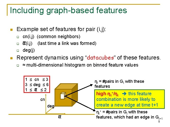
Including graph-based features n Example set of features for pair (i, j): q q q n cn(i, j) (common neighbors) ℓℓ(i, j) (last time a link was formed) deg(j) Represent dynamics using “datacubes” of these features. q ≈ multi-dimensional histogram on binned feature values 1 ≤ cn ≤ 3 3 ≤ deg ≤ 6 1 ≤ ℓℓ ≤ 2 ηt = #pairs in Gt with these features + high ηt /ηt this feature combination is more likely to create a new edge at time t+1 cn deg ℓℓ ηt+ = #pairs in Gt with these features, which had an edge in Gt+1 9

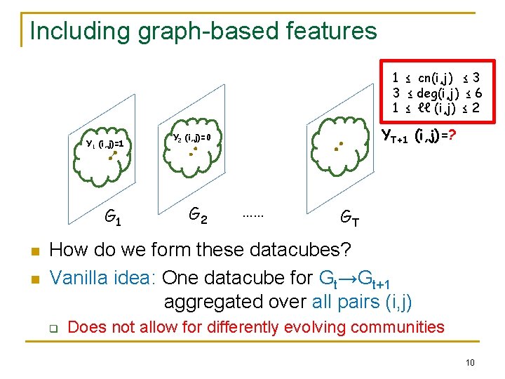
Including graph-based features 1 ≤ cn(i, j) ≤ 3 3 ≤ deg(i, j) ≤ 6 1 ≤ ℓℓ (i, j) ≤ 2 Y 1 (i, j)=1 G 1 n n YT+1 (i, j)=? Y 2 (i, j)=0 G 2 …… GT How do we form these datacubes? Vanilla idea: One datacube for Gt→Gt+1 aggregated over all pairs (i, j) q Does not allow for differently evolving communities 10

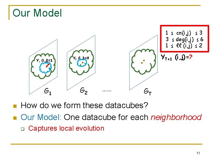
Our Model 1 ≤ cn(i, j) ≤ 3 3 ≤ deg(i, j) ≤ 6 1 ≤ ℓℓ (i, j) ≤ 2 Y 1 (i, j)=1 G 1 n n YT+1 (i, j)=? Y 2 (i, j)=0 G 2 …… GT How do we form these datacubes? Our Model: One datacube for each neighborhood q Captures local evolution 11

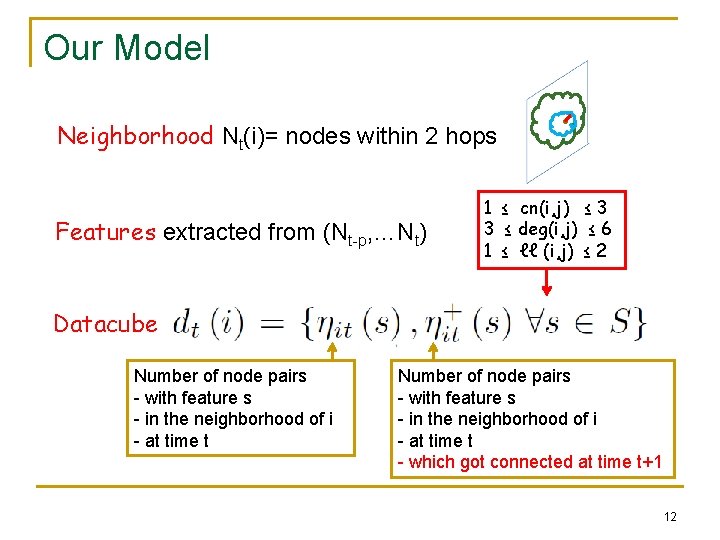
Our Model Neighborhood Nt(i)= nodes within 2 hops Features extracted from (Nt-p, …Nt) 1 ≤ cn(i, j) ≤ 3 3 ≤ deg(i, j) ≤ 6 1 ≤ ℓℓ (i, j) ≤ 2 Datacube Number of node pairs - with feature s - in the neighborhood of i - at time t - which got connected at time t+1 12

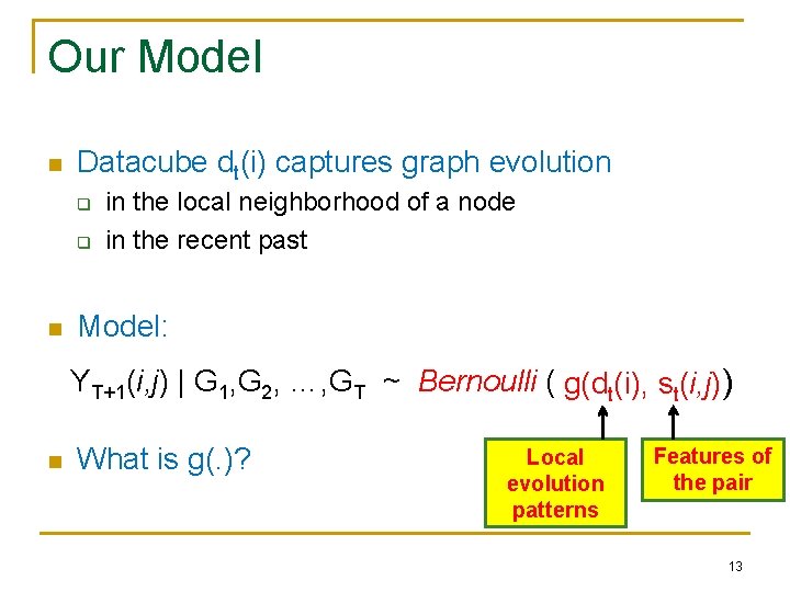
Our Model n Datacube dt(i) captures graph evolution q q n in the local neighborhood of a node in the recent past Model: YT+1(i, j) | G 1, G 2, …, GT ~ Bernoulli ( g (i, j)) g(d ) G 1, G 2, …GT t(i), st(i, j) n What is g(. )? Local evolution patterns Features of the pair 13

Outline n n n Model Estimator Consistency Scalability Experiments 14

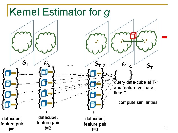
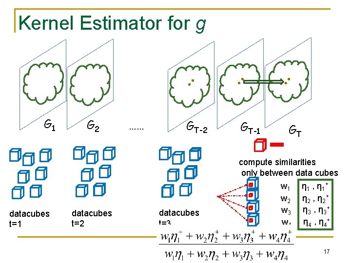
Kernel Estimator for g { { { datacube, feature pair t=2 { { GT-2 GT-1 GT {query data-cube at T-1 and feature vector at time T compute similarities … … datacube, feature pair t=1 …… { { { G 2 … { { G 1 datacube, feature pair t=3 15

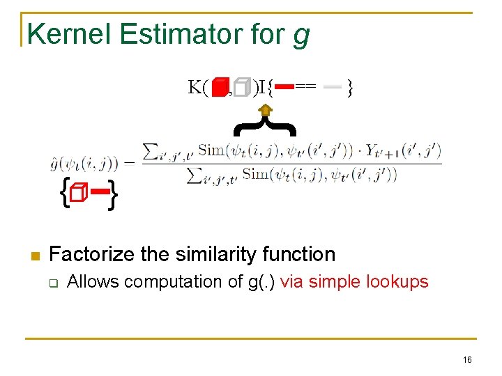
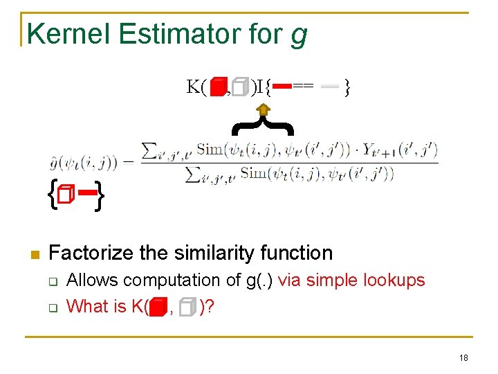
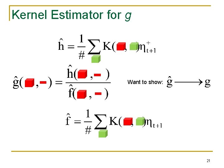
Kernel Estimator for g , )I{ == } } K( } n } Factorize the similarity function q Allows computation of g(. ) via simple lookups 16

Kernel Estimator for g G 1 G 2 …… GT-2 GT-1 GT compute similarities only between data cubes datacubes t=1 datacubes t=2 datacubes t=3 w 1 w 2 w 3 w 4 η 1 , η 1+ η 2 , η 2+ η 3 , η 3+ η 4 , η 4+ 17

Kernel Estimator for g , )I{ == } } K( } n } Factorize the similarity function q q Allows computation of g(. ) via simple lookups What is K( , )? 18

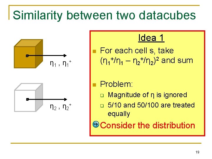
Similarity between two datacubes Idea 1 n For each cell s, take (η 1+/η 1 – η 2+/η 2)2 and sum n Problem: η 1 , η 1+ q η 2 , η 2+ q Magnitude of η is ignored 5/10 and 50/100 are treated equally Consider the distribution 19

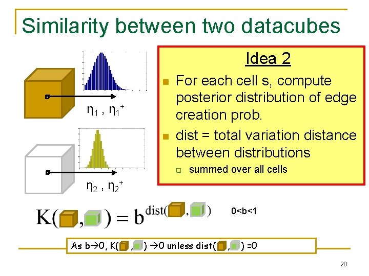
Similarity between two datacubes Idea 2 n η 1 , η 1+ n For each cell s, compute posterior distribution of edge creation prob. dist = total variation distance between distributions q summed over all cells η 2 , η 2+ 0<b<1 As b 0, K( , ) 0 unless dist( , ) =0 20

Kernel Estimator for g Want to show: 21

Outline n n n Model Estimator Consistency Scalability Experiments 22

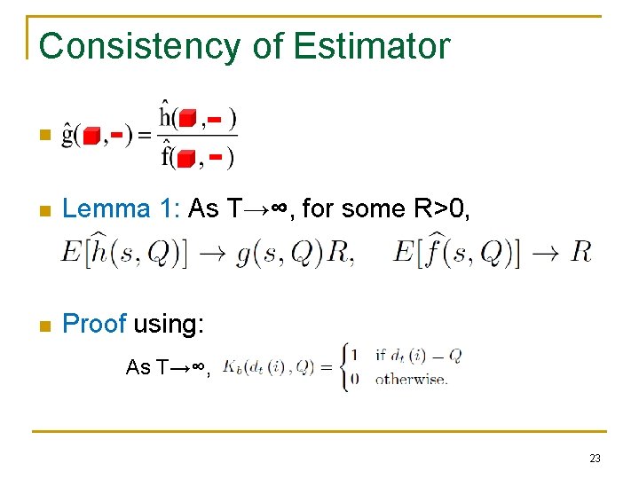
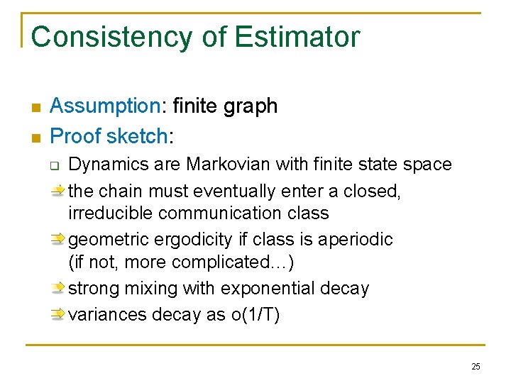
Consistency of Estimator n n Lemma 1: As T→∞, for some R>0, n Proof using: As T→∞, 23

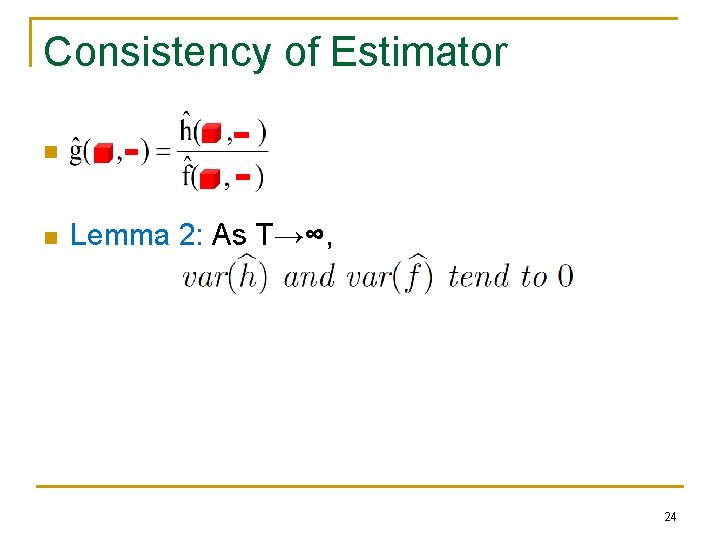
Consistency of Estimator n n Lemma 2: As T→∞, 24

Consistency of Estimator n n Assumption: finite graph Proof sketch: q Dynamics are Markovian with finite state space the chain must eventually enter a closed, irreducible communication class geometric ergodicity if class is aperiodic (if not, more complicated…) strong mixing with exponential decay variances decay as o(1/T) 25

Consistency of Estimator n Theorem: n Proof Sketch: q for some R>0 q So 26

Outline n n n Model Estimator Consistency Scalability Experiments 27

Scalability n Full solution: q q n Approximate solution: q n Summing over all n datacubes for all T timesteps Infeasible Sum over nearest neighbors of query datacube How do we find nearest neighbors? q Locality Sensitive Hashing (LSH) [Indyk+/98, Broder+/98] 28

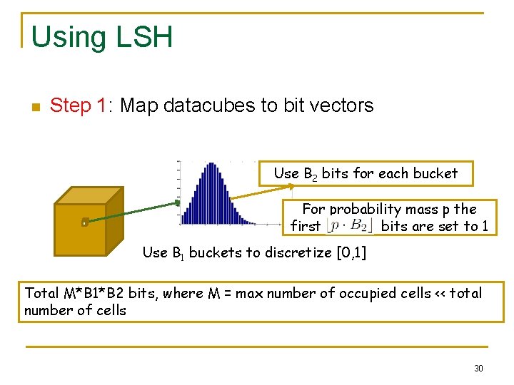
Using LSH n Devise a hashing function for datacubes such that q q “Similar” datacubes tend to be hashed to the same bucket “Similar” = small total variation distance between cells of datacubes 29

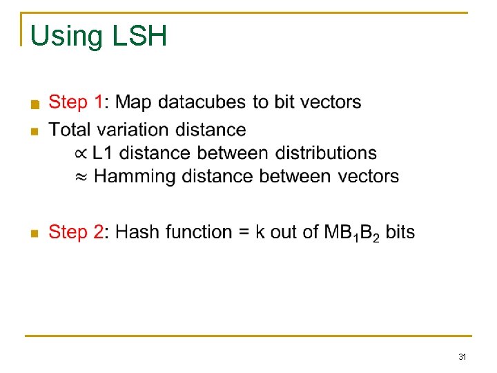
Using LSH n Step 1: Map datacubes to bit vectors Use B 2 bits for each bucket For probability mass p the first bits are set to 1 Use B 1 buckets to discretize [0, 1] Total M*B 1*B 2 bits, where M = max number of occupied cells << total number of cells 30

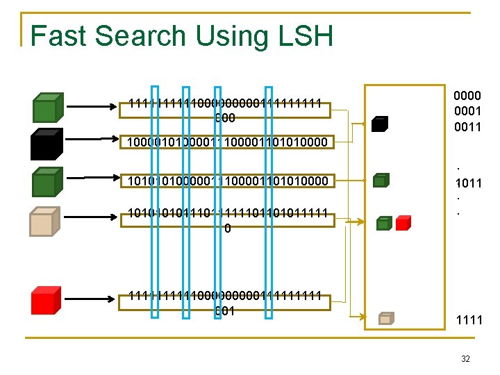
Using LSH n 31

Fast Search Using LSH 111110000011111 0000 0001 0011 1000010100001101010000011100001101010000 1010111011111101101011111 0 111110000011111 001 . . 1011. . 1111 32

Outline n n n Model Estimator Consistency Scalability Experiments 33

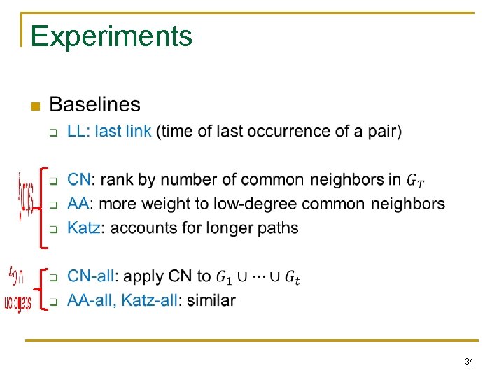
Experiments n 34

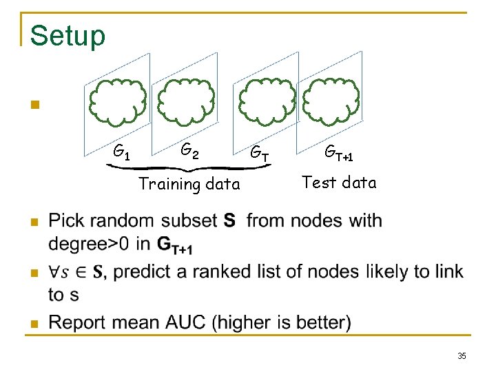
Setup n G 1 G 2 Training data GT GT+1 Test data 35

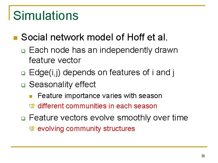
Simulations n Social network model of Hoff et al. q q q Each node has an independently drawn feature vector Edge(i, j) depends on features of i and j Seasonality effect n q Feature importance varies with season different communities in each season Feature vectors evolve smoothly over time evolving community structures 36

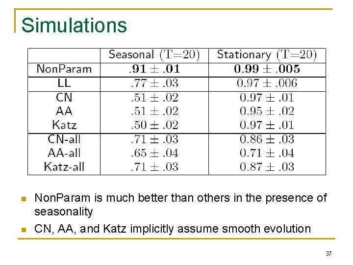
Simulations n n Non. Param is much better than others in the presence of seasonality CN, AA, and Katz implicitly assume smooth evolution 37

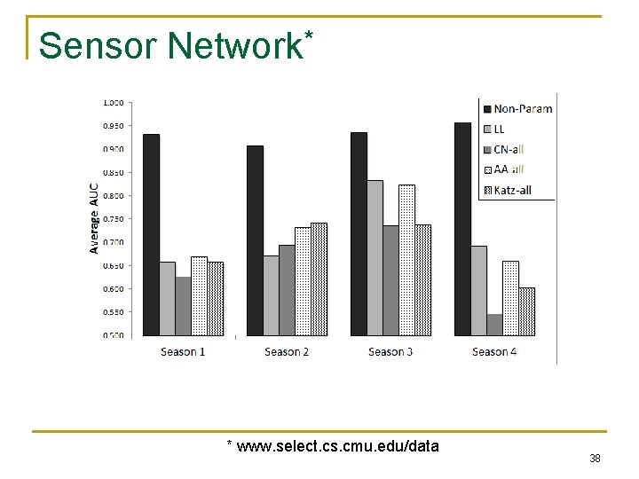
Sensor Network* * www. select. cs. cmu. edu/data 38

Summary n Link formation is assumed to depend on q q n Admits a kernel-based estimator q q n the neighborhood’s evolution over a time window Consistency Scalability via LSH Works particularly well for q q Seasonal effects differently evolving communities 39