Nonparametric Econometrics Seminar Estimating the Term Structure of

Nonparametric Econometrics Seminar Estimating the Term Structure of Interest Rates for Thai Government Bonds: A B-Spline Approach Kant Thamchamrassri February 5, 2006 1

Introduction n Interest rate in modern financial theories q q q n Fixed income market (bonds and derivative securities) Other market securities (for time discounting) Corporate investment decisions (alternative opportunities and cost of capital) The term structure of interest rates q q Representing relationship between bond yields and maturities Useful in pricing coupon bonds Introduction 2

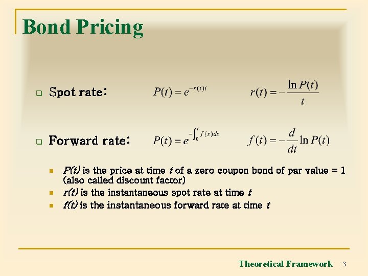
Bond Pricing q Spot rate: q Forward rate: n P(t) is the price at time t of a zero coupon bond of par value = 1 n (also called discount factor) r(t) is the instantaneous spot rate at time t f(t) is the instantaneous forward rate at time t n Theoretical Framework 3

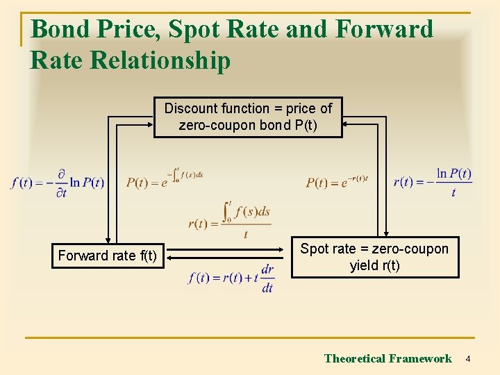
Bond Price, Spot Rate and Forward Rate Relationship Discount function = price of zero-coupon bond P(t) Forward rate f(t) Spot rate = zero-coupon yield r(t) Theoretical Framework 4

Methods for Extracting the Term Structure n n n Simple linear regression Polynomial splines Exponential splines Basis splines (B-splines) Nelson and Siegel (1985) and its variants Bootstrapping and cubic splines Theoretical Framework 5

Splines q q Spline is a statistical technique and a form of a linear non-parametric interpolation method. A kth-order spline is a piecewise polynomial approximation with k-degree polynomials. A yield curve can be estimated using many polynomial splines connected at arbitrary selected points called knot points. Some conditions are applied: continuity and differentiability Theoretical Framework 6

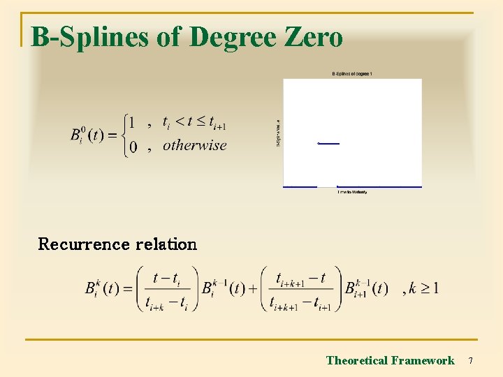
B-Splines of Degree Zero Recurrence relation Theoretical Framework 7

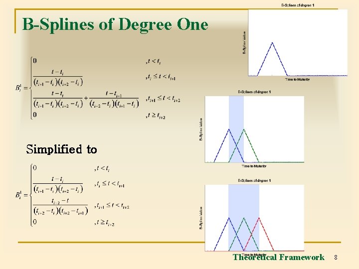
B-Splines of Degree One Simplified to Theoretical Framework 8

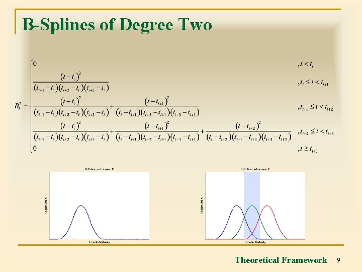
B-Splines of Degree Two Theoretical Framework 9

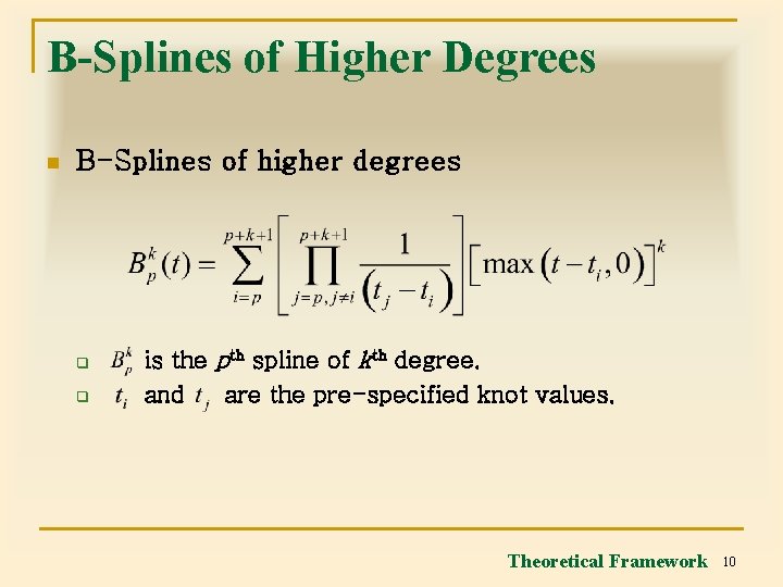
B-Splines of Higher Degrees n B-Splines of higher degrees q q is the pth spline of kth degree. and are the pre-specified knot values. Theoretical Framework 10

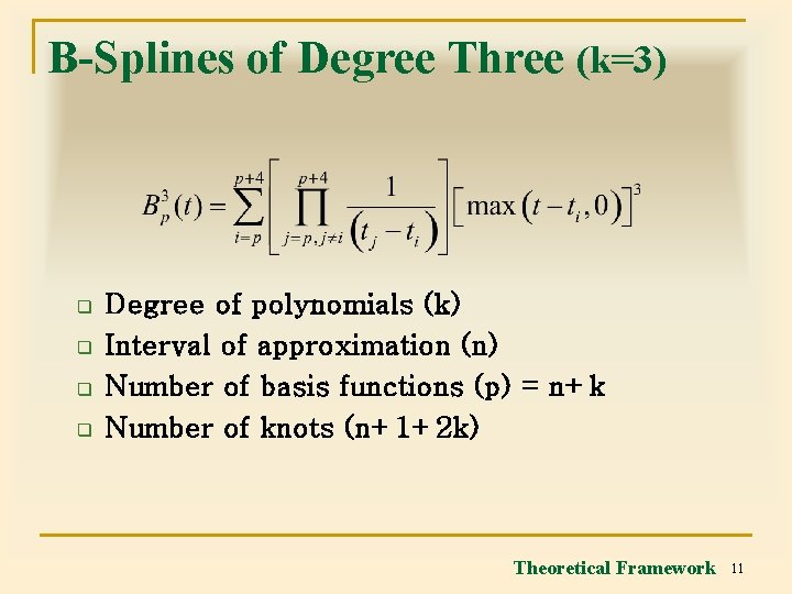
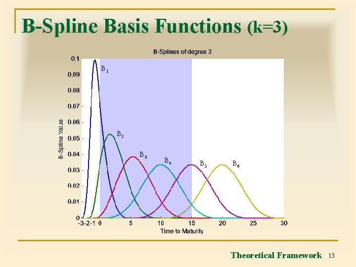
B-Splines of Degree Three (k=3) q q Degree of polynomials (k) Interval of approximation (n) Number of basis functions (p) = n+k Number of knots (n+1+2 k) Theoretical Framework 11

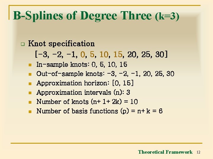
B-Splines of Degree Three (k=3) q Knot specification [-3, -2, -1, 0, 5, 10, 15, 20, 25, 30] n n n In-sample knots: 0, 5, 10, 15 Out-of-sample knots: -3, -2, -1, 20, 25, 30 Approximation horizon: [0, 15] Approximation intervals (n): 3 Number of knots (n+1+2 k) = 10 Number of basis functions (p) = n+k = 6 Theoretical Framework 12

B-Spline Basis Functions (k=3) B 1 B 2 B 3 B 4 B 5 B 6 Theoretical Framework 13

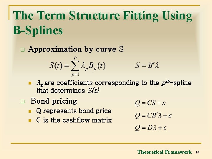
The Term Structure Fitting Using B-Splines q Approximation by curve S n q λp are coefficients corresponding to the pth-spline that determines S(t) Bond pricing n n Q represents bond price C is the cashflow matrix Theoretical Framework 14

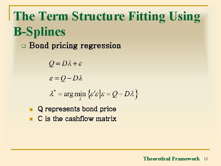
The Term Structure Fitting Using B-Splines q Bond pricing regression n n Q represents bond price C is the cashflow matrix Theoretical Framework 15

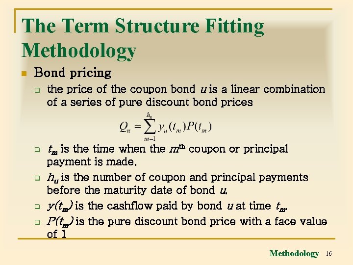
The Term Structure Fitting Methodology n Bond pricing q q q the price of the coupon bond u is a linear combination of a series of pure discount bond prices tm is the time when the mth coupon or principal payment is made. hu is the number of coupon and principal payments before the maturity date of bond u. y(tm) is the cashflow paid by bond u at time tm. P(tm) is the pure discount bond price with a face value of 1 Methodology 16

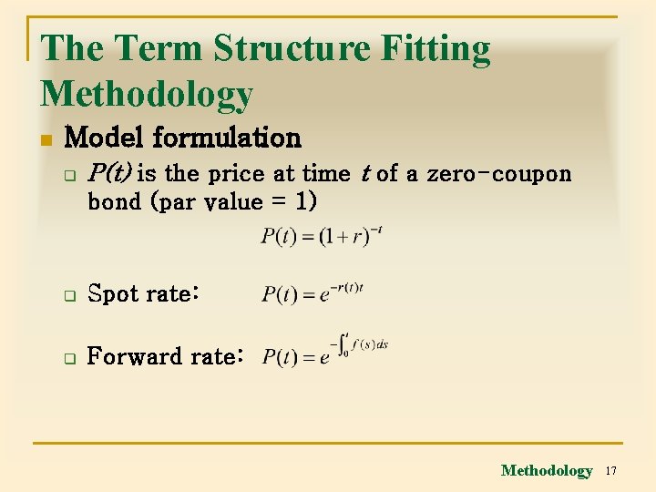
The Term Structure Fitting Methodology n Model formulation q P(t) is the price at time t of a zero-coupon bond (par value = 1) q Spot rate: q Forward rate: Methodology 17

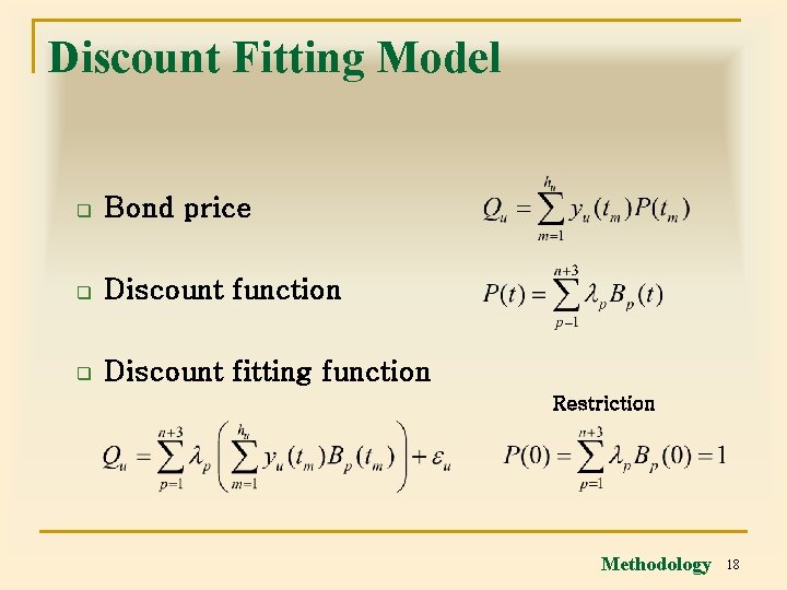
Discount Fitting Model q Bond price q Discount function q Discount fitting function Restriction Methodology 18

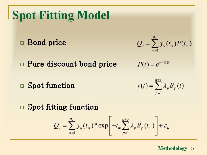
Spot Fitting Model q Bond price q Pure discount bond price q Spot function q Spot fitting function Methodology 19

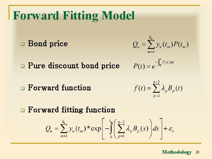
Forward Fitting Model q Bond price q Pure discount bond price q Forward function q Forward fitting function Methodology 20

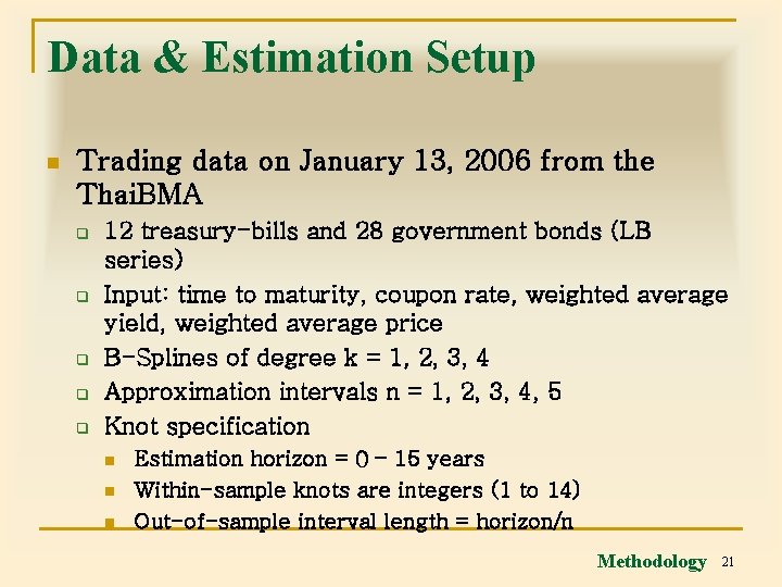
Data & Estimation Setup n Trading data on January 13, 2006 from the Thai. BMA q q q 12 treasury-bills and 28 government bonds (LB series) Input: time to maturity, coupon rate, weighted average yield, weighted average price B-Splines of degree k = 1, 2, 3, 4 Approximation intervals n = 1, 2, 3, 4, 5 Knot specification n Estimation horizon = 0 – 15 years Within-sample knots are integers (1 to 14) Out-of-sample interval length = horizon/n Methodology 21

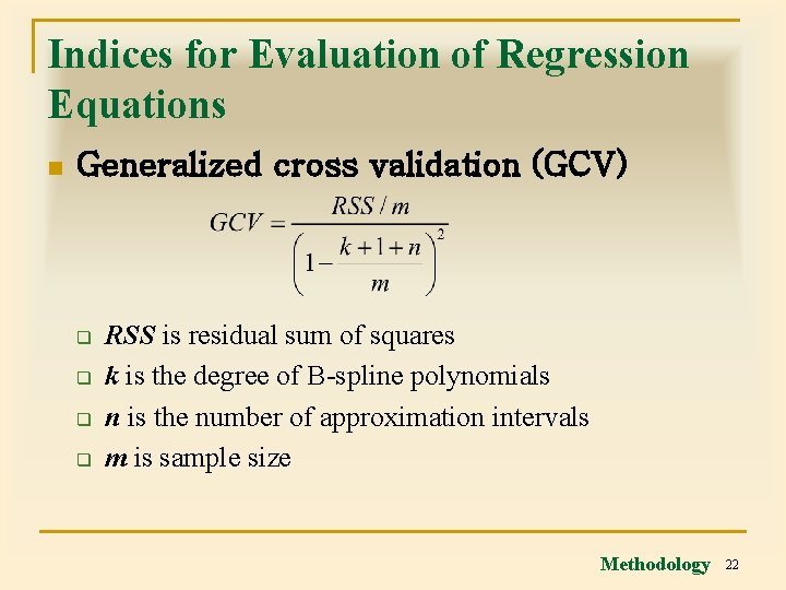
Indices for Evaluation of Regression Equations n Generalized cross validation (GCV) q q RSS is residual sum of squares k is the degree of B-spline polynomials n is the number of approximation intervals m is sample size Methodology 22

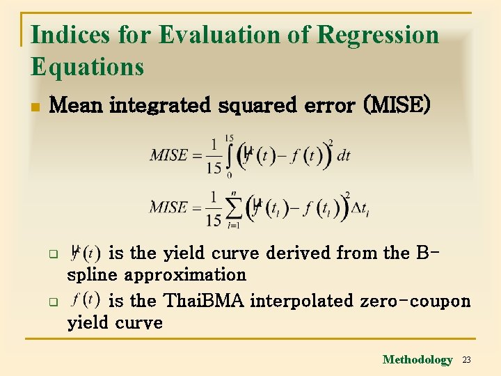
Indices for Evaluation of Regression Equations n Mean integrated squared error (MISE) q q is the yield curve derived from the Bspline approximation is the Thai. BMA interpolated zero-coupon yield curve Methodology 23

Estimated Results n n n Generalized cross validation (GCV) Mean integrated squared error (MISE) Comparison with the Thai. BMA Empirical Results 24

Minimum Values of Generalized Cross Validation (GCV) Empirical Results 25

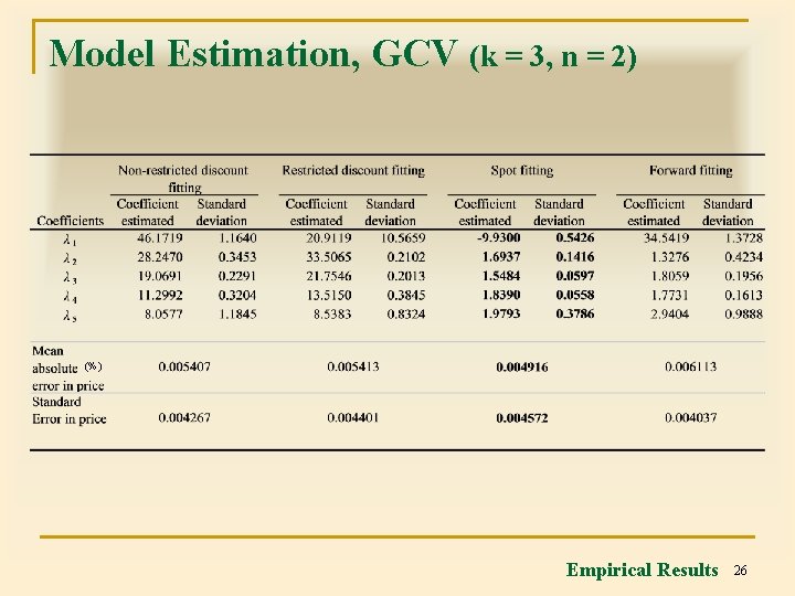
Model Estimation, GCV (k = 3, n = 2) (%) Empirical Results 26

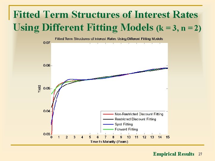
Fitted Term Structures of Interest Rates Using Different Fitting Models (k = 3, n = 2) Empirical Results 27

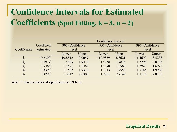
Confidence Intervals for Estimated Coefficients (Spot Fitting, k = 3, n = 2) Note. * denotes statistical significance at 1% level. Empirical Results 28

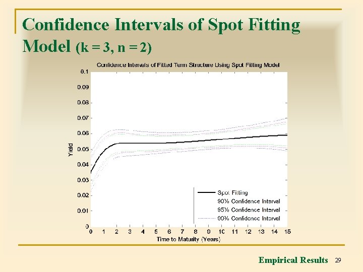
Confidence Intervals of Spot Fitting Model (k = 3, n = 2) Empirical Results 29

Minimum Values of Mean Integrated Squared Error (MISE) Empirical Results 30

Model Estimation, MISE (k = 3, n = 3) (%) Empirical Results 31

Fitted Term Structures of Interest Rates Using Different Fitting Models (k = 3, n = 3) Empirical Results 32

Confidence Intervals for Estimated Coefficients (Restricted Discount Fitting, k = 3, n = 2) Note. * denotes statistical significance at 1% level. Empirical Results 33

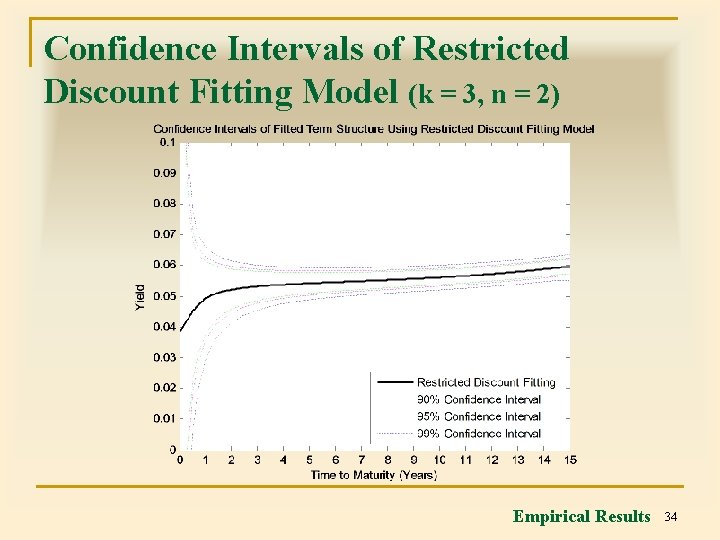
Confidence Intervals of Restricted Discount Fitting Model (k = 3, n = 2) Empirical Results 34

Fitted term structures: GCV, MISE in Comparison to the Thai. BMA Yield Curve Empirical Results 35

Confidence Intervals of Restricted Discount Fitting/ Spot Fitting with Thai. BMA Spot Fitting (GCV) Restricted Discount Fitting (MISE) Empirical Results 36

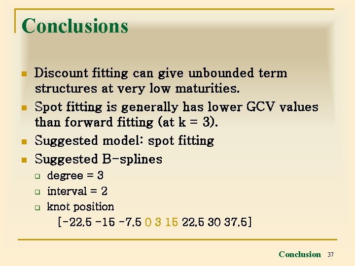
Conclusions n n Discount fitting can give unbounded term structures at very low maturities. Spot fitting is generally has lower GCV values than forward fitting (at k = 3). Suggested model: spot fitting Suggested B-splines q q q degree = 3 interval = 2 knot position [-22. 5 -15 -7. 5 0 3 15 22. 5 30 37. 5] Conclusion 37