NonLinear Modelling and Chaotic Neural Networks Evolutionary and

Non-Linear Modelling and Chaotic Neural Networks Evolutionary and Neural Computing Group Cardiff University SBRN 2000

Overview • • • The Freeman model The Gamma Test Non-Linear Modelling Delayed Feedback Control Synchronisation

The Freeman Model • Freeman [1991] studied the olfactory bulb of rabbits • In the rest state, the dynamics of this neural cluster are chaotic • When presented with a familiar scent, the neural system rapidly simplifies its behaviour • The dynamics then become more orderly, more nearly periodic than when in the rest state

Questions. . . • How can we construct chaotic neural networks? • How can we control such networks so that they stabilise onto an unstable periodic orbit (characteristic of the applied stimulus) when a stimulus is presented? • We are looking for biologically plausible mechanisms

The Gamma Test Principal Contributors Antonia J Jones Ana Oliveria Nenad Končar Steve Margetts Aðalbjörn Stefánsson Peter Durrant Alban Tsui Dafydd Evans www. cs. cf. ac. uk/wingamma

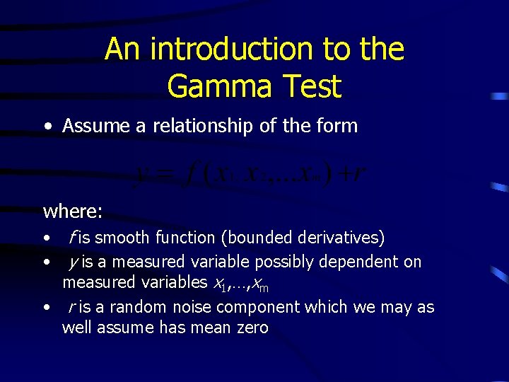
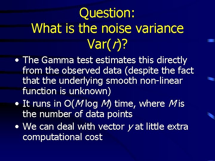
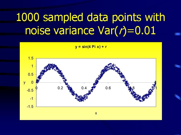
An introduction to the Gamma Test • Assume a relationship of the form where: • f is smooth function (bounded derivatives) • y is a measured variable possibly dependent on measured variables x 1, …, xm • r is a random noise component which we may as well assume has mean zero

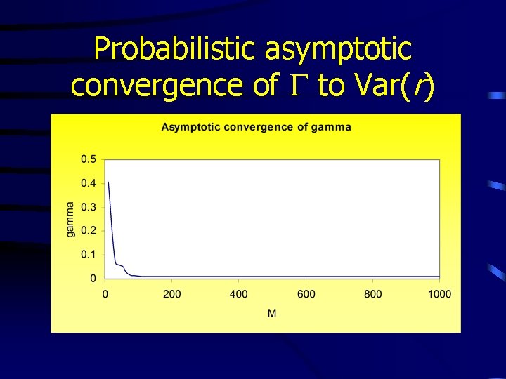
Question: What is the noise variance Var(r)? • The Gamma test estimates this directly from the observed data (despite the fact that the underlying smooth non-linear function is unknown) • It runs in O(M log M) time, where M is the number of data points • We can deal with vector y at little extra computational cost

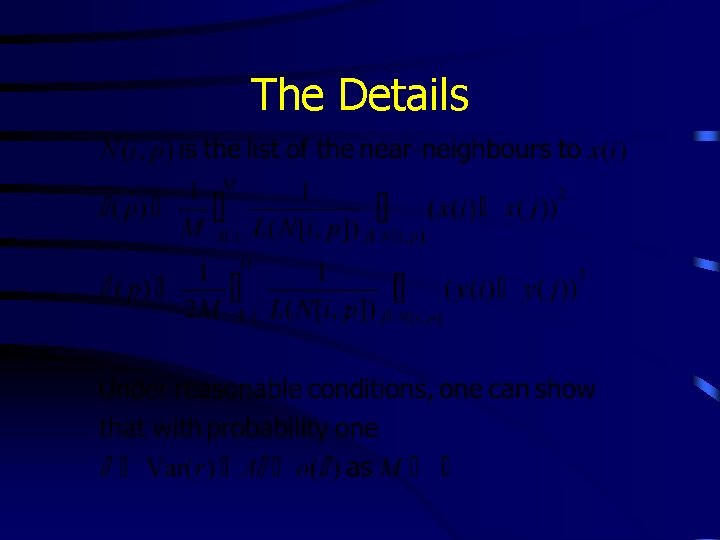
The Details

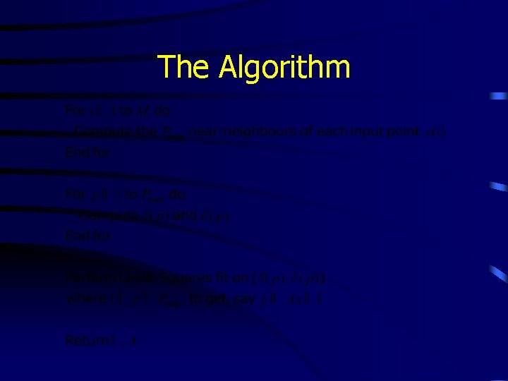
The Algorithm

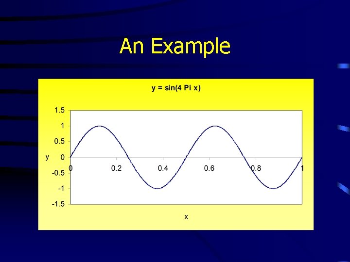
An Example

1000 sampled data points with noise variance Var(r)=0. 01

Probabilistic asymptotic convergence of G to Var(r)

Using The Gamma Test for Non-Linear Modelling • Embedding Dimension • Irregular Embeddings • Modelling a particular chaotic system

Question: What use is the Gamma Test? • We can calculate the embedding dimension – the number of past values required to calculate the next point • We can compute irregular embeddings – the best combination of past values for a given embedding dimension

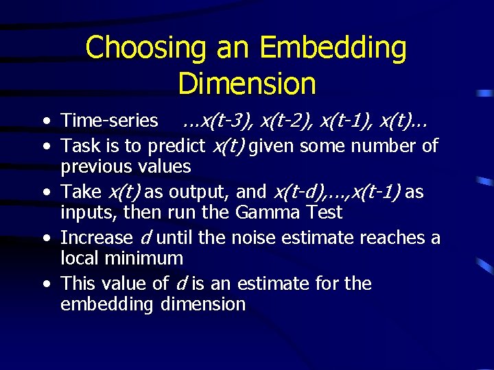
Choosing an Embedding Dimension • Time-series. . . x(t-3), x(t-2), x(t-1), x(t). . . • Task is to predict x(t) given some number of previous values • Take x(t) as output, and x(t-d), . . . , x(t-1) as inputs, then run the Gamma Test • Increase d until the noise estimate reaches a local minimum • This value of d is an estimate for the embedding dimension

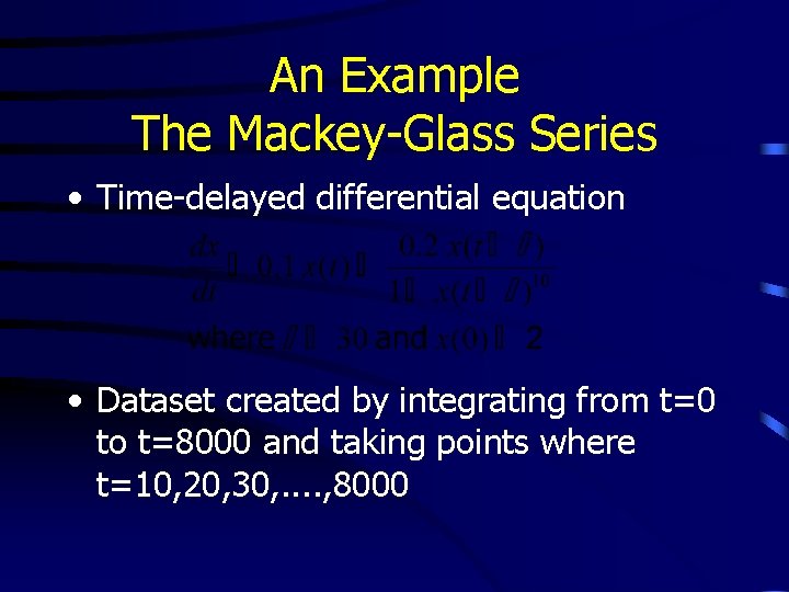
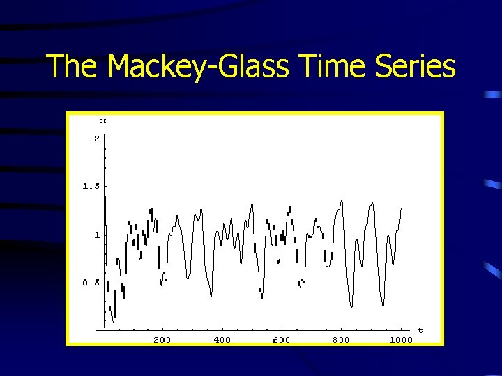
An Example The Mackey-Glass Series • Time-delayed differential equation • Dataset created by integrating from t=0 to t=8000 and taking points where t=10, 20, 30, . . , 8000

The Mackey-Glass Time Series

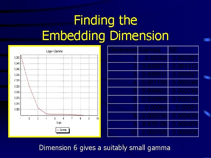
Finding the Embedding Dimension 6 gives a suitably small gamma

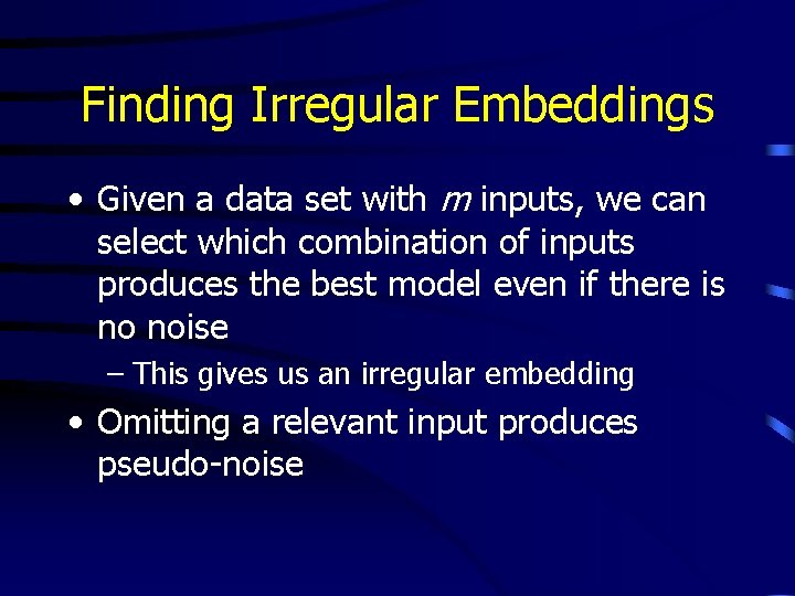
Finding Irregular Embeddings • Given a data set with m inputs, we can select which combination of inputs produces the best model even if there is no noise – This gives us an irregular embedding • Omitting a relevant input produces pseudo-noise

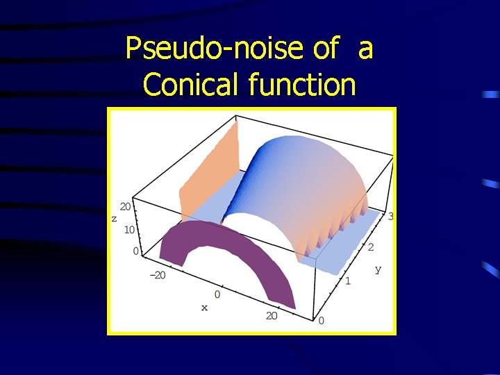
Pseudo-noise of a Conical function

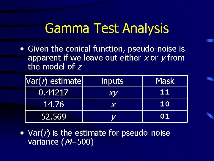
Gamma Test Analysis • Given the conical function, pseudo-noise is apparent if we leave out either x or y from the model of z Var(r) estimate 0. 44217 14. 76 52. 569 inputs xy x y Mask 11 10 01 • Var(r) is the estimate for pseudo-noise variance (M=500)

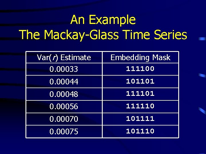
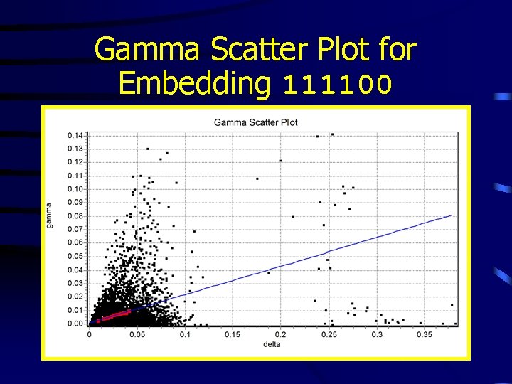
An Example The Mackay-Glass Time Series Var(r) Estimate 0. 00033 Embedding Mask 111100 0. 00044 101101 0. 00048 111101 0. 00056 111110 0. 00070 101111 0. 00075 101110

Gamma Scatter Plot for Embedding 111100

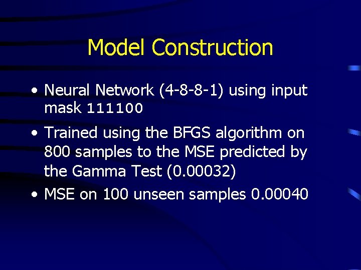
Model Construction • Neural Network (4 -8 -8 -1) using input mask 111100 • Trained using the BFGS algorithm on 800 samples to the MSE predicted by the Gamma Test (0. 00032) • MSE on 100 unseen samples 0. 00040

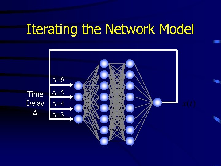
Iterating the Network Model D=6 Time Delay D D=5 D=4 D=3

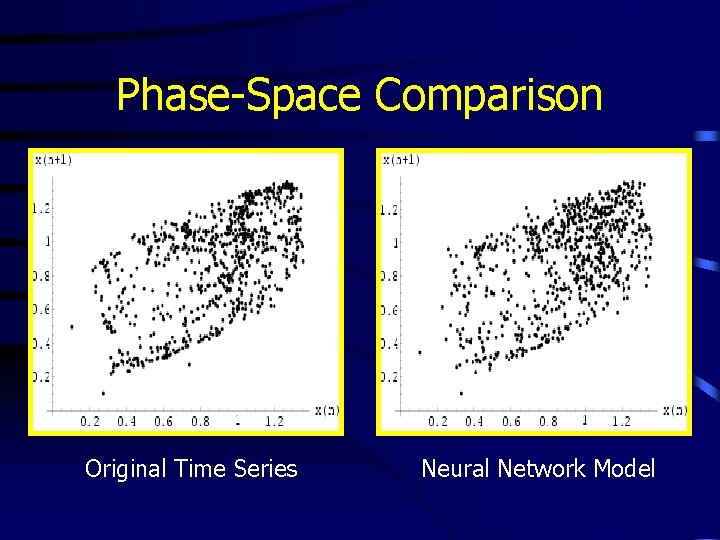
Phase-Space Comparison Original Time Series Neural Network Model

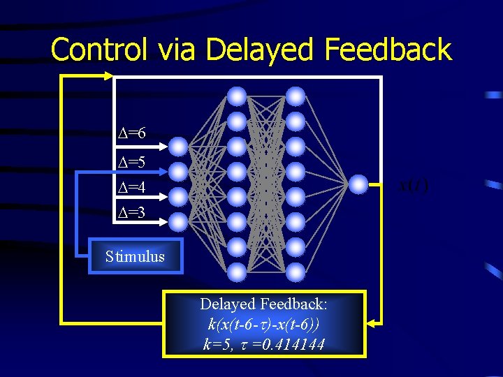
Control via Delayed Feedback D=6 D=5 D=4 D=3 Stimulus Delayed Feedback: k(x(t-6 -t)-x(t-6)) k=5, t =0. 414144

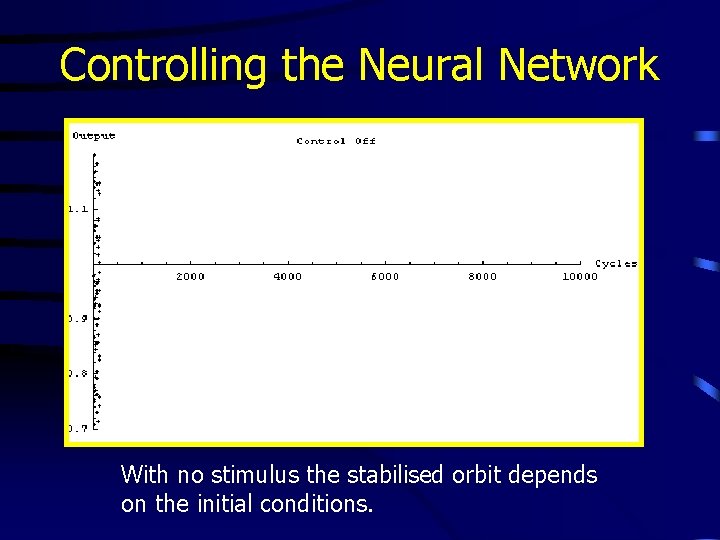
Controlling the Neural Network With no stimulus the stabilised orbit depends on the initial conditions.

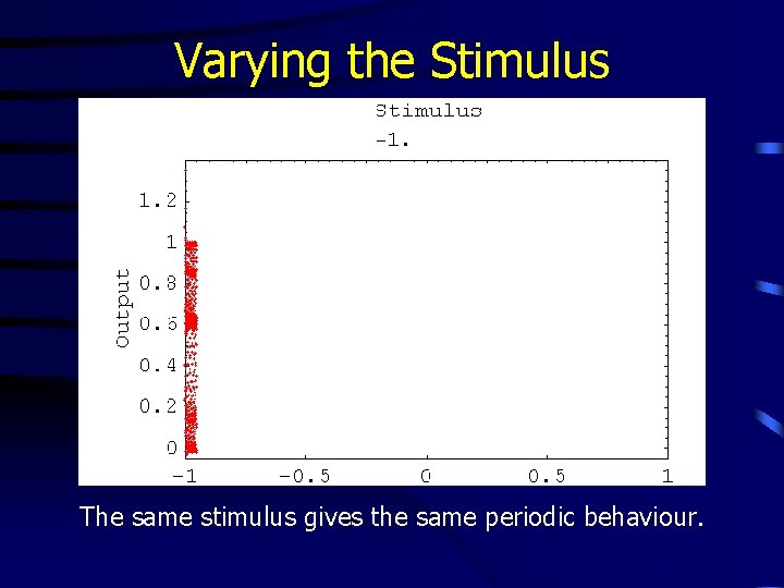
Varying the Stimulus The same stimulus gives the same periodic behaviour.

A Generic Model for a Chaotic Neural Network

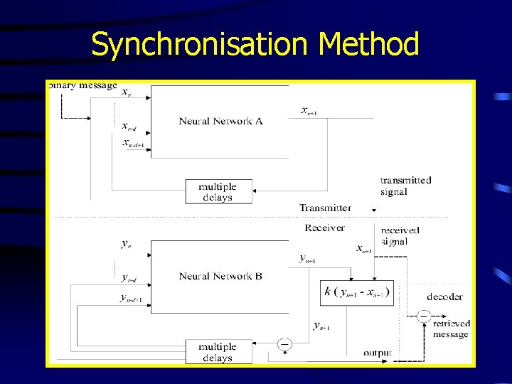
Synchronisation Method

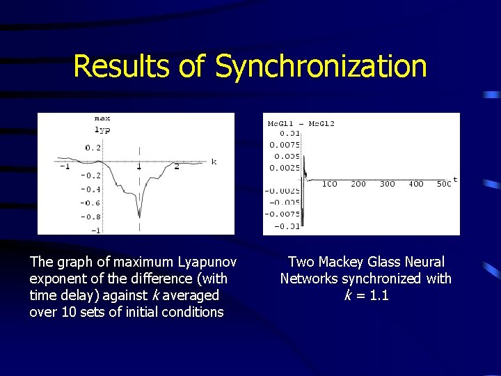
Results of Synchronization The graph of maximum Lyapunov exponent of the difference (with time delay) against k averaged over 10 sets of initial conditions Two Mackey Glass Neural Networks synchronized with k = 1. 1

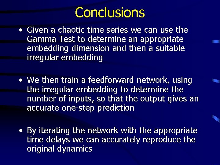
Conclusions • Given a chaotic time series we can use the Gamma Test to determine an appropriate embedding dimension and then a suitable irregular embedding • We then train a feedforward network, using the irregular embedding to determine the number of inputs, so that the output gives an accurate one-step prediction • By iterating the network with the appropriate time delays we can accurately reproduce the original dynamics

The significance of time delayed feedback • Finally by adding a time delayed feedback (activated in the presence of a stimulus) we can stabilise the iterative network onto an unstable periodic orbit • The particular orbit stabilised depends on the applied stimulus • The entire artificial neural system accurately reproduces the phenomenon described by Freeman

Synchronisation • Results shown by Skarda and Freeman [Skarda 1987] support the hypothesis that neural dynamics are heavily dependent on chaotic activity • Nowadays it is believed that synchronization plays a crucial role in information processing in living organisms and could lead to important applications in speech and image processing [Ogorzallek 1993] • We have shown that time delayed feedback also offers a biologically plausible mechanism for neural synchronisation

SBRN 2000 Group Picture