Nonlinear function estimation Topics Function approximation Parameter estimation

Nonlinear function estimation Topics • Function approximation • Parameter estimation • Classes of models • Choice of complexity in functional relationships • Bias-Variance tradeoffs • Considerations in model selection

Readings Hastie, Tibshirani and Friedman, 2001. � Chapter 1 and 2. 1 -2. 2 for terminology � 2. 3 Least Squares vs Nearest Neighbors � 2. 4 Statistical decision theory. Formal basis. * 2. 5 Curse of dimensionality ** 2. 6 General Function approximation * 2. 7 - 2. 8 Structured approaches, Restricting complexity, Error tradeoffs � 3. 3. 1 -3. 3 Linear regression review ** 6. 6. 1 -6. 4 Kernel Regression methods � Background, *Important, **Essential

Terminology Statistical Learning Function estimation Training set Calibration data Learner Model Supervised Learning Fit to observed outcomes

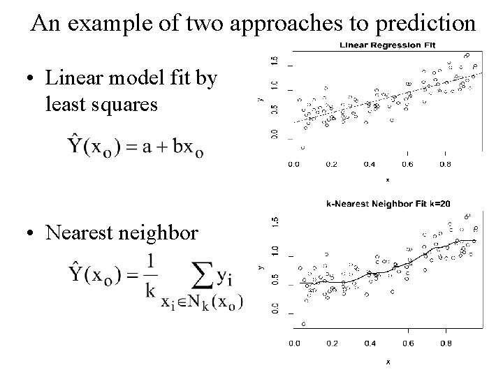
An example of two approaches to prediction • Linear model fit by least squares • Nearest neighbor

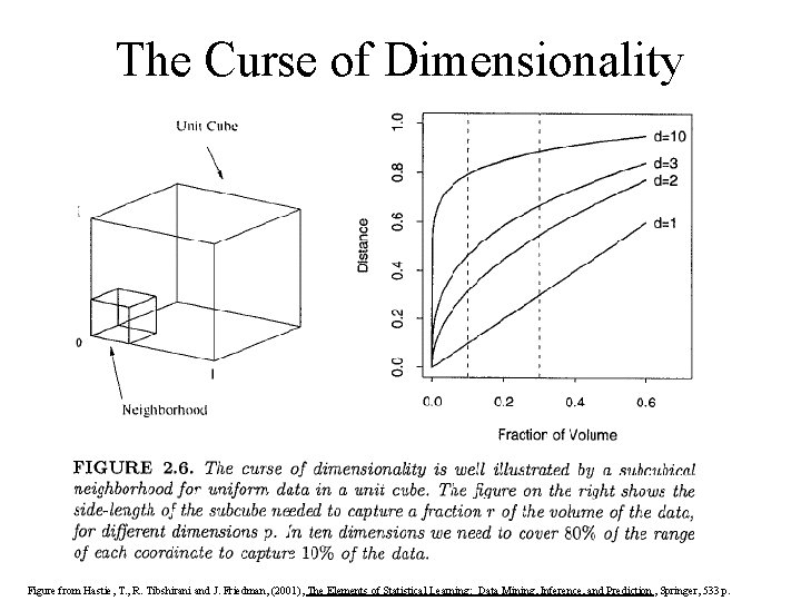
The Curse of Dimensionality Figure from Hastie, T. , R. Tibshirani and J. Friedman, (2001), The Elements of Statistical Learning: Data Mining, Inference, and Prediction , Springer, 533 p.

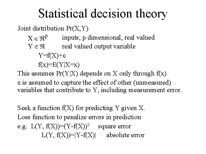
Statistical decision theory Joint distribution Pr(X, Y) inputs, p dimensional, real valued output variable Y=f(X)+ f(x)=E(Y|X=x) This assumes Pr(Y|X) depends on X only through f(x) is assumed to capture the effect of other (unmeasured) variables that contribute to Y, including measurement error. Seek a function f(X) for predicting Y given X. Loss function to penalize errors in prediction e. g. L(Y, f(X))=(Y-f(X))2 square error L(Y, f(X))=|Y-f(X)| absolute error

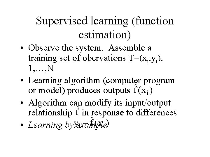
Supervised learning (function estimation) • Observe the system. Assemble a training set of obervations T=(xi, yi), 1, …, N • Learning algorithm (computer program or model) produces outputs • Algorithm can modify its input/output relationship in response to differences • Learning by example

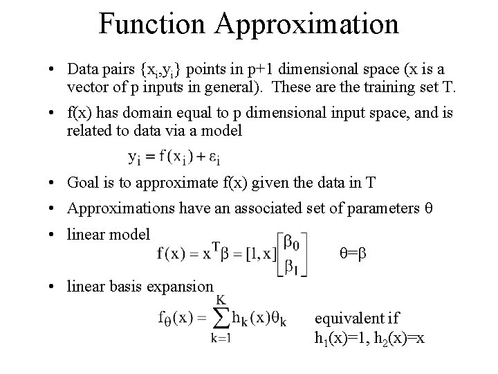
Function Approximation • Data pairs {xi, yi} points in p+1 dimensional space (x is a vector of p inputs in general). These are the training set T. • f(x) has domain equal to p dimensional input space, and is related to data via a model • Goal is to approximate f(x) given the data in T • Approximations have an associated set of parameters • linear model = • linear basis expansion equivalent if h 1(x)=1, h 2(x)=x

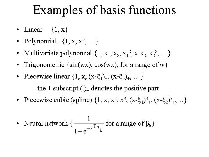
Examples of basis functions • Linear {1, x} • Polynomial {1, x, x 2, …} • Multivariate polynomial {1, x 2, x 1 x 2, x 22, …} • Trigonometric {sin(wx), cos(wx), for a range of w} • Piecewise linear {1, x, (x- 1)+, (x- 2)+, …} the + subscript (. )+ denotes the positive part • Piecewise cubic (spline) {1, x, x 2, x 3, (x- 1)3+, (x- 2)3+, …} • Neural network { for a range of k}

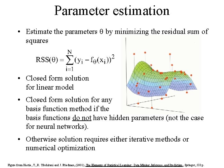
Parameter estimation • Estimate the parameters by minimizing the residual sum of squares • Closed form solution for linear model • Closed form solution for any basis function method if the basis functions do not have hidden parameters (not the case for neural networks). • Otherwise solution requires either iterative methods or numerical optimization Figure from Hastie, T. , R. Tibshirani and J. Friedman, (2001), The Elements of Statistical Learning: Data Mining, Inference, and Prediction , Springer, 533 p.

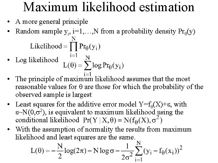
Maximum likelihood estimation • A more general principle • Random sample yi, i=1, …, N from a probability density Pr (y) • Log likelihood • The principle of maximum likelihood assumes that the most reasonable values for are those for which the probability of the observed sample is largest • Least squares for the additive error model Y=f (X)+ , with ~N(0, 2), is equivalent to maximum likelihood using the conditional likelihood • With the assumption of normality the results from maximum likelihood and least squares are the same.

Classes of Models used to Represent the Relationships Between Variables Beyond linear fit by least squares or nearest neighbor approach

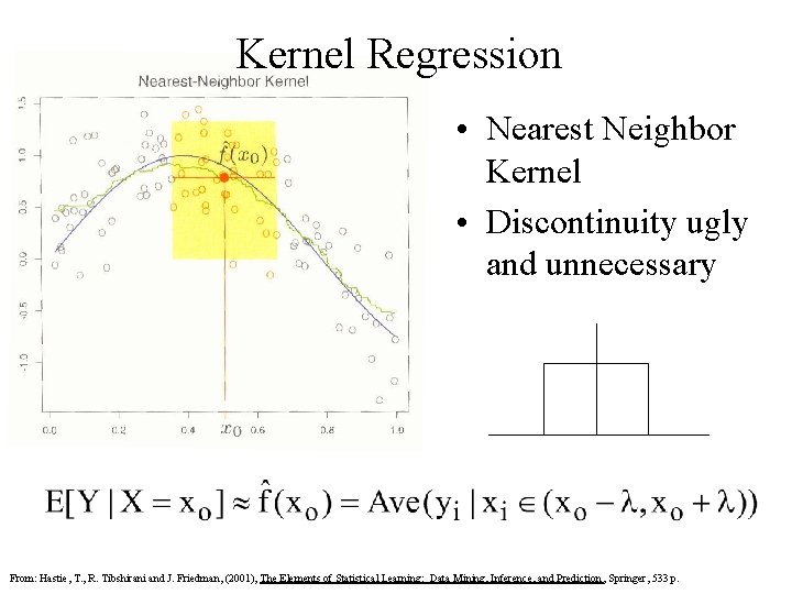
Kernel Regression • Nearest Neighbor Kernel • Discontinuity ugly and unnecessary From: Hastie, T. , R. Tibshirani and J. Friedman, (2001), The Elements of Statistical Learning: Data Mining, Inference, and Prediction , Springer, 533 p.

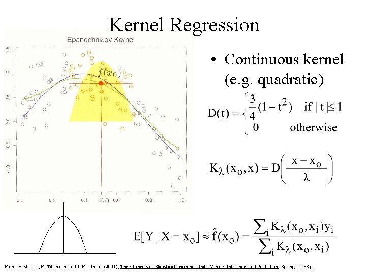
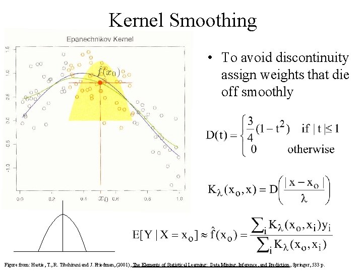
Kernel Regression • Continuous kernel (e. g. quadratic) From: Hastie, T. , R. Tibshirani and J. Friedman, (2001), The Elements of Statistical Learning: Data Mining, Inference, and Prediction , Springer, 533 p.

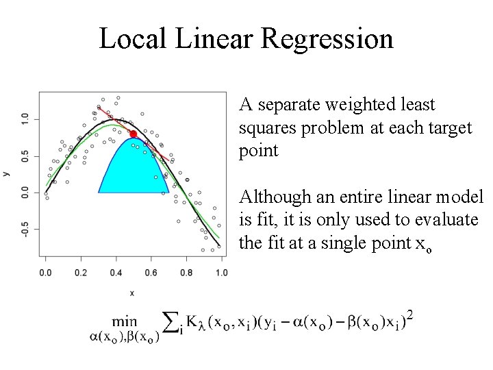
Local Linear Regression A separate weighted least squares problem at each target point Although an entire linear model is fit, it is only used to evaluate the fit at a single point xo

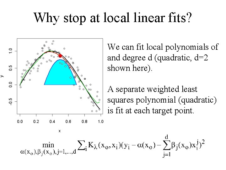
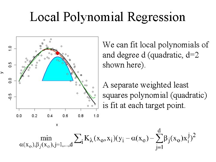
Why stop at local linear fits? We can fit local polynomials of and degree d (quadratic, d=2 shown here). A separate weighted least squares polynomial (quadratic) is fit at each target point.

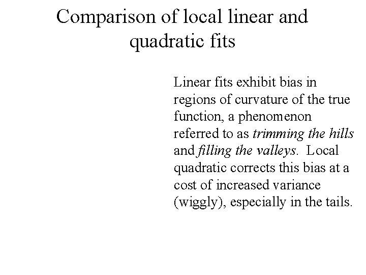
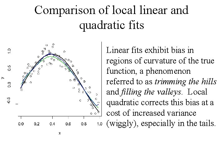
Comparison of local linear and quadratic fits Linear fits exhibit bias in regions of curvature of the true function, a phenomenon referred to as trimming the hills and filling the valleys. Local quadratic corrects this bias at a cost of increased variance (wiggly), especially in the tails.

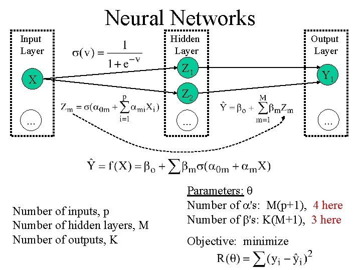
Neural Networks Input Layer X Hidden Layer Z 1 Output Layer Y 1 Z 2. . . Number of inputs, p Number of hidden layers, M Number of outputs, K . . . Parameters: Number of 's: M(p+1), 4 here Number of 's: K(M+1), 3 here Objective: minimize

Neural network function fit • The model is generally overparameterized and the optimization problem is nonconvex and unstable with multiple local minima. • Use global optimization methodology from a number of random start configurations. • Average predictions over a collection of better solutions.

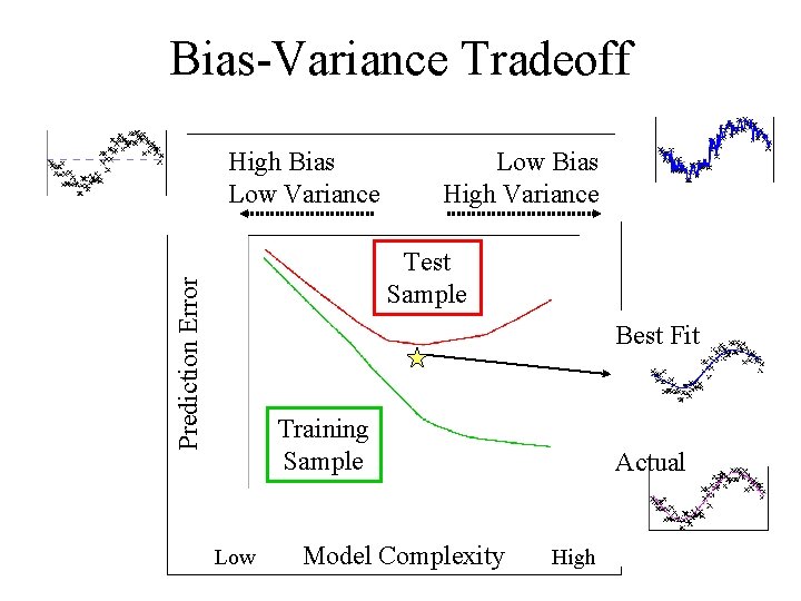
Considerations in Model Selection • Choice of complexity in functional relationship – Theoretically infinite choice • Interplay between bias, variance and model complexity – Interpolation versus function fitting • The generalization performance of a learning method relates to its prediction capability on independent test data.

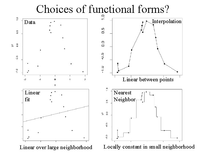
Choices of functional forms? Interpolation Data Linear between points Linear fit Linear over large neighborhood Nearest Neighbor Locally constant in small neighborhood

The actual functional relationship (random noise added to realization of points)

Bias-Variance Tradeoff High Bias Low Variance Low Bias High Variance Prediction Error Test Sample Best Fit Training Sample Low Model Complexity Actual High

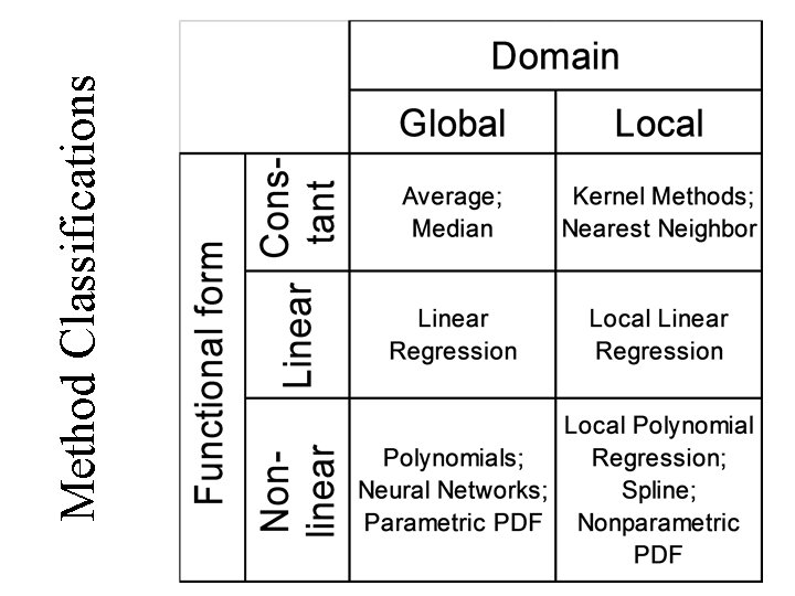
Method Classifications

Kernel Smoothers and Local Regression • • Kernel Smoothing Local Linear Regression Local Polynomial Regression Local Regression in High Dimensions **Hastie, Tibshirani and Friedman Chapter 6, sections 6. 1 -6. 4

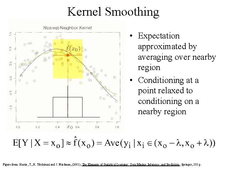
Kernel Smoothing • Expectation approximated by averaging over nearby region • Conditioning at a point relaxed to conditioning on a nearby region Figure from: Hastie, T. , R. Tibshirani and J. Friedman, (2001), The Elements of Statistical Learning: Data Mining, Inference, and Prediction , Springer, 533 p.

Kernel Smoothing • To avoid discontinuity assign weights that die off smoothly Figure from: Hastie, T. , R. Tibshirani and J. Friedman, (2001), The Elements of Statistical Learning: Data Mining, Inference, and Prediction , Springer, 533 p.

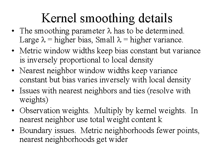
Kernel smoothing details • The smoothing parameter has to be determined. Large = higher bias, Small = higher variance. • Metric window widths keep bias constant but variance is inversely proportional to local density • Nearest neighbor window widths keep variance constant but bias varies inversely with local density • Issues with nearest neighbors and ties (resolve with weights) • Observation weights. Multiply by kernel weights. In nearest neighbor use total weight content k • Boundary issues. Metric neighborhoods fewer points, nearest neighborhoods get wider

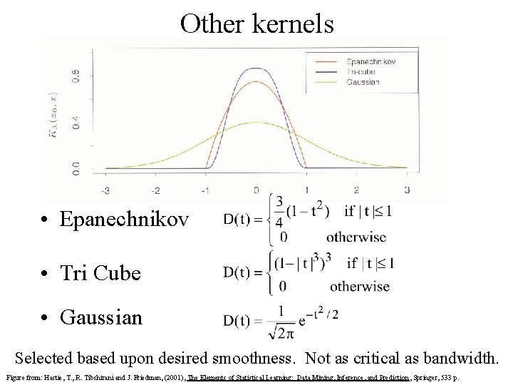
Other kernels • Epanechnikov • Tri Cube • Gaussian Selected based upon desired smoothness. Not as critical as bandwidth. Figure from: Hastie, T. , R. Tibshirani and J. Friedman, (2001), The Elements of Statistical Learning: Data Mining, Inference, and Prediction , Springer, 533 p.

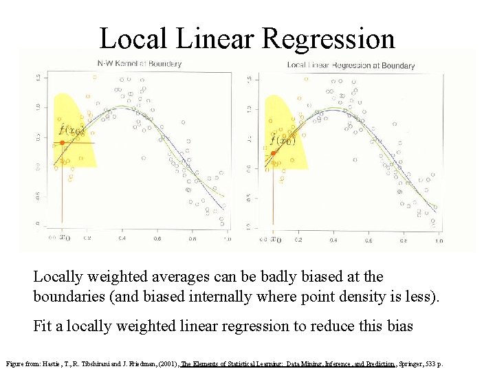
Local Linear Regression Locally weighted averages can be badly biased at the boundaries (and biased internally where point density is less). Fit a locally weighted linear regression to reduce this bias Figure from: Hastie, T. , R. Tibshirani and J. Friedman, (2001), The Elements of Statistical Learning: Data Mining, Inference, and Prediction , Springer, 533 p.

Local Linear Regression A separate weighted least squares problem at each target point Although an entire linear model is fit, it is only used to evaluate the fit at a single point xo

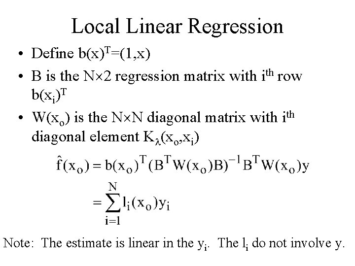
Local Linear Regression • Define b(x)T=(1, x) • B is the N 2 regression matrix with row b(xi)T • W(xo) is the N N diagonal matrix with diagonal element K (xo, xi) Note: The estimate is linear in the yi. The li do not involve y.

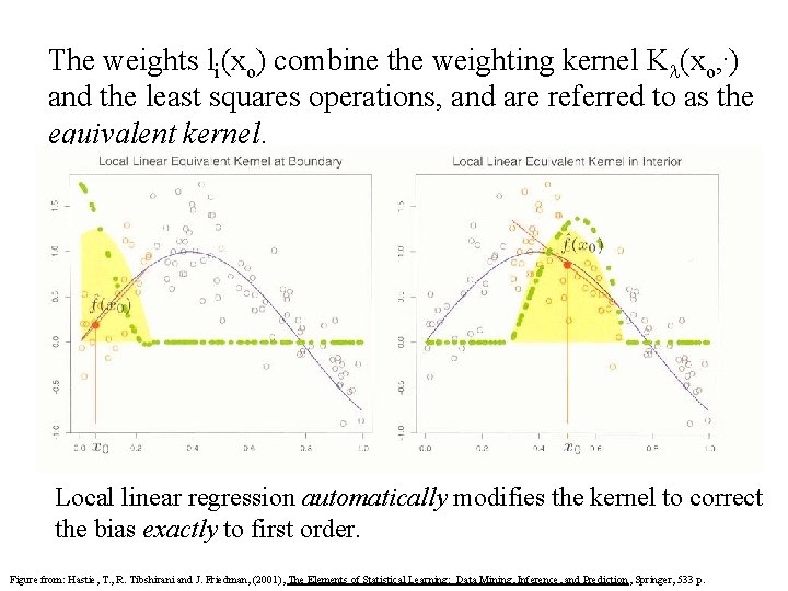
The weights li(xo) combine the weighting kernel K (xo, ) and the least squares operations, and are referred to as the equivalent kernel. Local linear regression automatically modifies the kernel to correct the bias exactly to first order. Figure from: Hastie, T. , R. Tibshirani and J. Friedman, (2001), The Elements of Statistical Learning: Data Mining, Inference, and Prediction , Springer, 533 p.

Local Polynomial Regression We can fit local polynomials of and degree d (quadratic, d=2 shown here). A separate weighted least squares polynomial (quadratic) is fit at each target point.

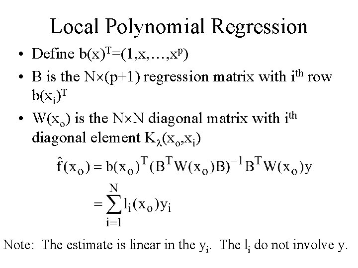
Local Polynomial Regression • Define b(x)T=(1, x, …, xp) • B is the N (p+1) regression matrix with row b(xi)T • W(xo) is the N N diagonal matrix with diagonal element K (xo, xi) Note: The estimate is linear in the yi. The li do not involve y.

Comparison of local linear and quadratic fits Linear fits exhibit bias in regions of curvature of the true function, a phenomenon referred to as trimming the hills and filling the valleys. Local quadratic corrects this bias at a cost of increased variance (wiggly), especially in the tails.

Hastie et al. , 2001's collected wisdom • Local linear fits can help bias dramatically at the boundaries at a modest cost in variance. Local quadratic fits do little at the boundaries for bias, but increase variance a lot. • Local quadratic fits tend to be most helpful in reducing bias due to curvature in the interior of the domain. • Asymptotic analysis suggests that local polynomials of odd degree dominate those of even degree. This is largely due to the domination of MSE by boundary effects.

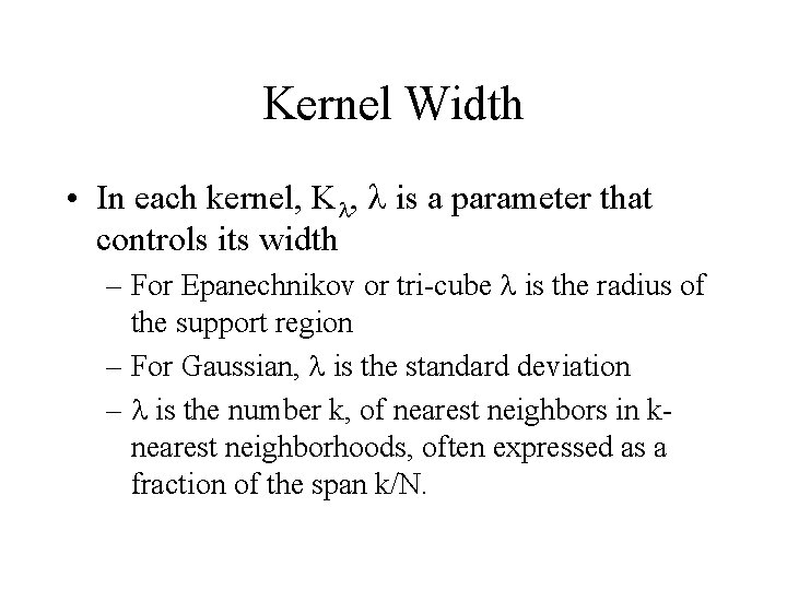
Kernel Width • In each kernel, K , is a parameter that controls its width – For Epanechnikov or tri-cube is the radius of the support region – For Gaussian, is the standard deviation – is the number k, of nearest neighbors in knearest neighborhoods, often expressed as a fraction of the span k/N.

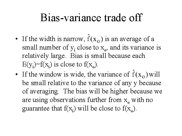
Bias-variance trade off • If the width is narrow, is an average of a small number of yi close to xo, and its variance is relatively large. Bias is small because each E(yi)=f(xi) is close to f(xo). • If the window is wide, the variance of will be small relative to the variance of any y because of averaging. The bias will be higher because we are using observations further from xo with no guarantee that f(xi) will be close to f(xo).

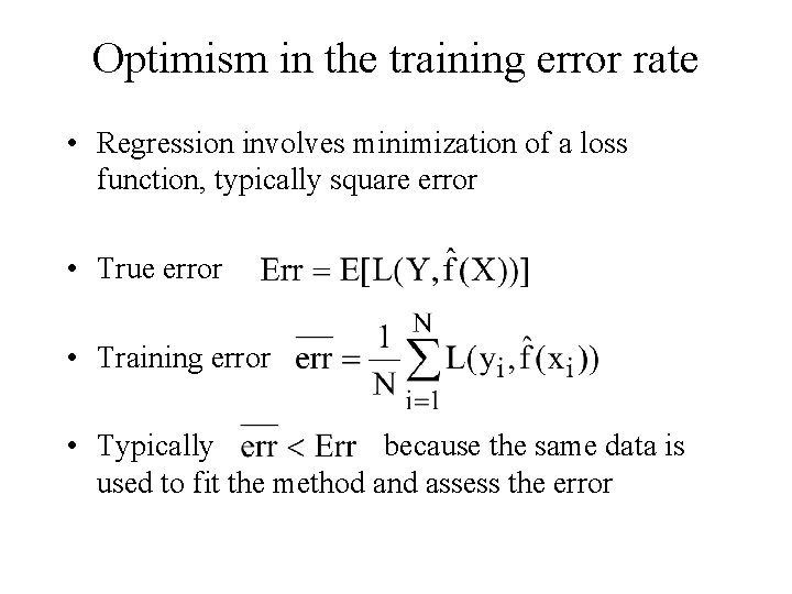
Optimism in the training error rate • Regression involves minimization of a loss function, typically square error • True error • Training error • Typically because the same data is used to fit the method and assess the error

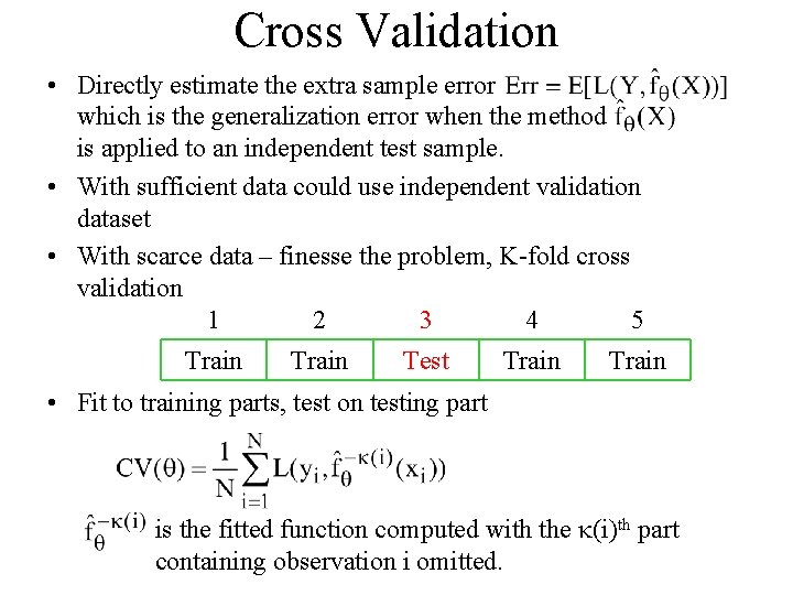
Cross Validation • Directly estimate the extra sample error which is the generalization error when the method is applied to an independent test sample. • With sufficient data could use independent validation dataset • With scarce data – finesse the problem, K-fold cross validation 1 2 3 4 5 Train Test Train • Fit to training parts, test on testing part is the fitted function computed with the (i)th part containing observation i omitted.

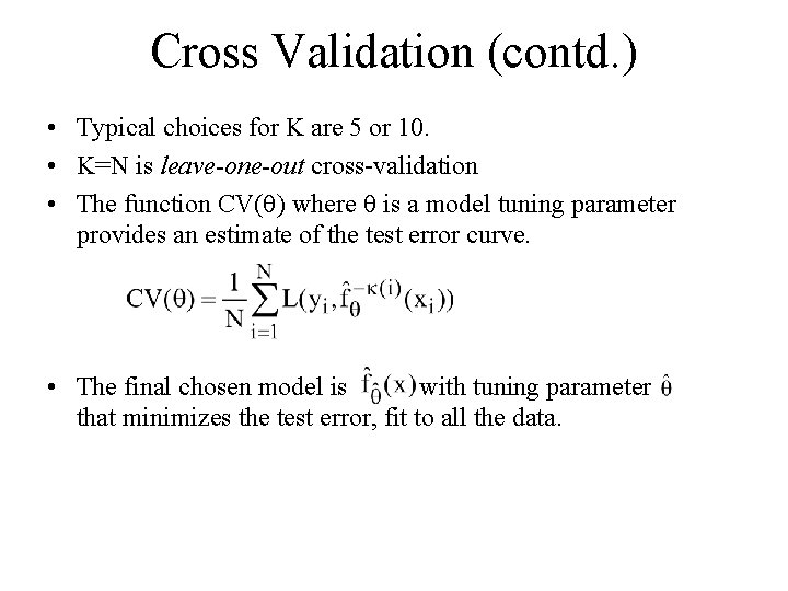
Cross Validation (contd. ) • Typical choices for K are 5 or 10. • K=N is leave-one-out cross-validation • The function CV( ) where is a model tuning parameter provides an estimate of the test error curve. • The final chosen model is with tuning parameter that minimizes the test error, fit to all the data.

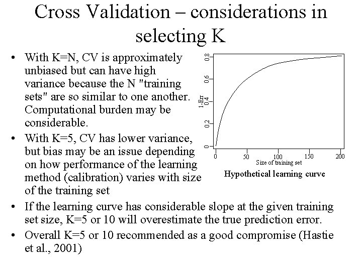
Cross Validation – considerations in selecting K 0 0. 2 1 -Err 0. 4 0. 6 0. 8 • With K=N, CV is approximately unbiased but can have high variance because the N "training sets" are so similar to one another. Computational burden may be considerable. • With K=5, CV has lower variance, but bias may be an issue depending 150 0 200 100 50 Size of training set on how performance of the learning Hypothetical learning curve method (calibration) varies with size of the training set • If the learning curve has considerable slope at the given training set size, K=5 or 10 will overestimate the true prediction error. • Overall K=5 or 10 recommended as a good compromise (Hastie et al. , 2001)