Nonlinear classifiers Neural networks Linear classifiers on pixels

Non-linear classifiers Neural networks

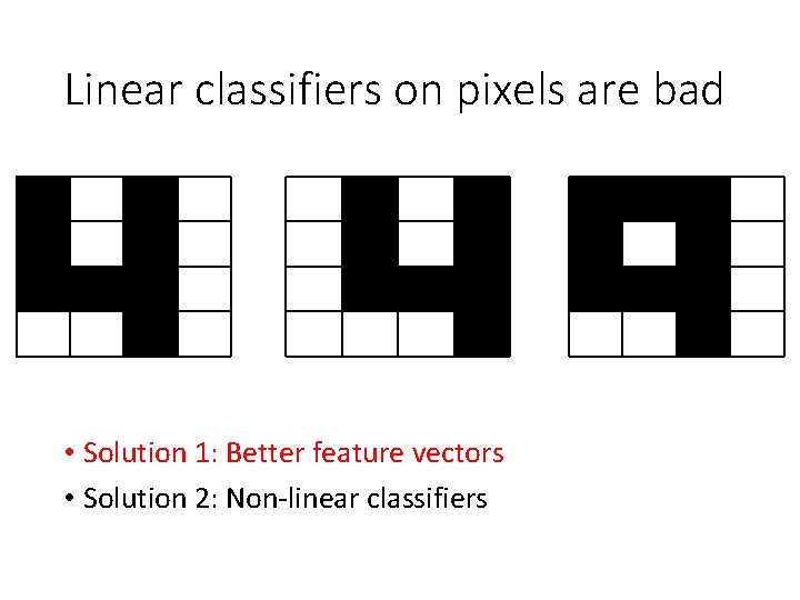
Linear classifiers on pixels are bad • Solution 1: Better feature vectors • Solution 2: Non-linear classifiers

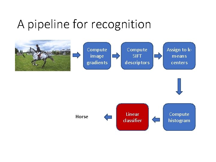
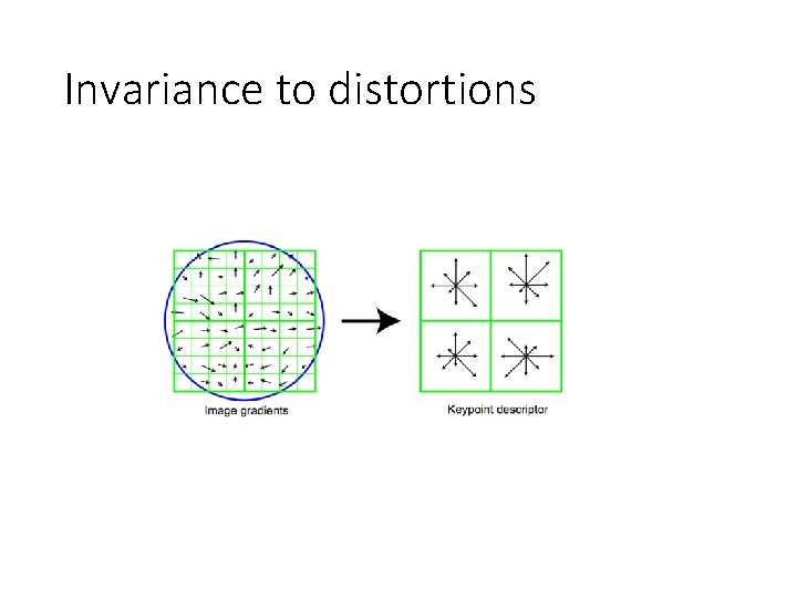
A pipeline for recognition Compute image gradients Horse Compute SIFT descriptors Linear classifier Assign to kmeans centers Compute histogram

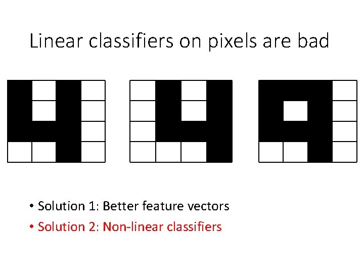
Linear classifiers on pixels are bad • Solution 1: Better feature vectors • Solution 2: Non-linear classifiers

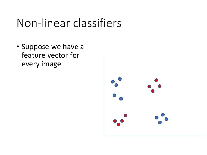
Non-linear classifiers • Suppose we have a feature vector for every image

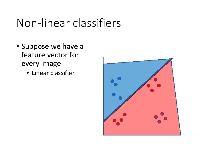
Non-linear classifiers • Suppose we have a feature vector for every image • Linear classifier

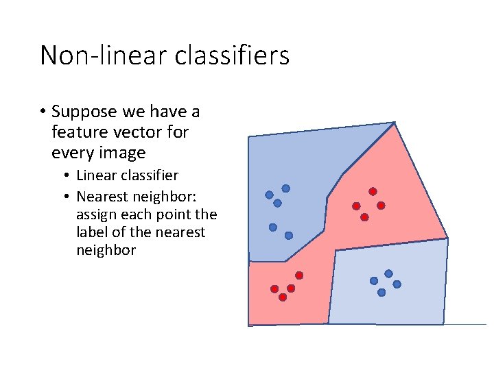
Non-linear classifiers • Suppose we have a feature vector for every image • Linear classifier • Nearest neighbor: assign each point the label of the nearest neighbor

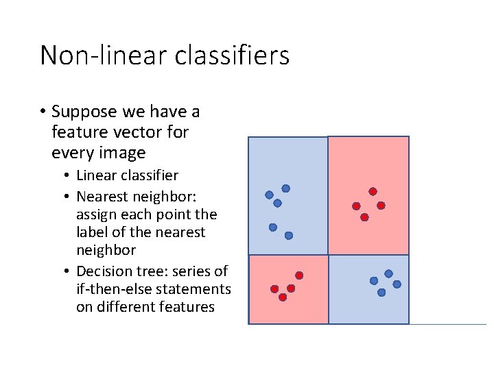
Non-linear classifiers • Suppose we have a feature vector for every image • Linear classifier • Nearest neighbor: assign each point the label of the nearest neighbor • Decision tree: series of if-then-else statements on different features

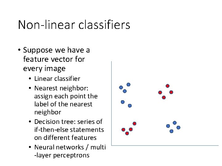
Non-linear classifiers • Suppose we have a feature vector for every image • Linear classifier • Nearest neighbor: assign each point the label of the nearest neighbor • Decision tree: series of if-then-else statements on different features • Neural networks / multi -layer perceptrons

A pipeline for recognition Compute image gradients Horse Compute SIFT descriptors Linear classifier Assign to kmeans centers Compute histogram

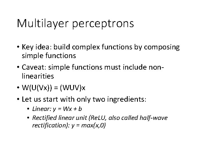
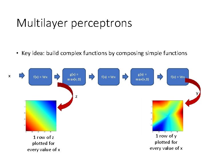
Multilayer perceptrons • Key idea: build complex functions by composing simple functions • Caveat: simple functions must include nonlinearities • W(U(Vx)) = (WUV)x • Let us start with only two ingredients: • Linear: y = Wx + b • Rectified linear unit (Re. LU, also called half-wave rectification): y = max(x, 0)

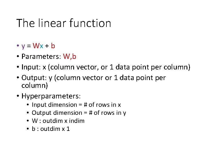
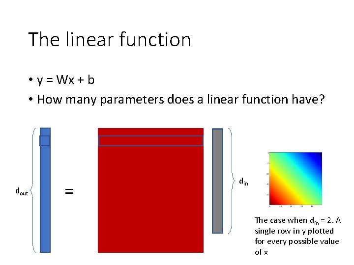
The linear function • y = Wx + b • Parameters: W, b • Input: x (column vector, or 1 data point per column) • Output: y (column vector or 1 data point per column) • Hyperparameters: • • Input dimension = # of rows in x Output dimension = # of rows in y W : outdim x indim b : outdim x 1

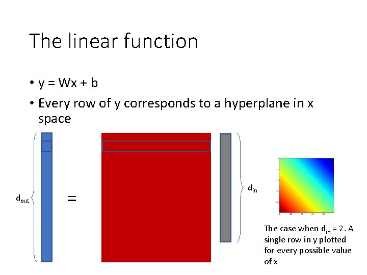
The linear function • y = Wx + b • Every row of y corresponds to a hyperplane in x space dout = din The case when din = 2. A single row in y plotted for every possible value of x

Multilayer perceptrons • Key idea: build complex functions by composing simple functions x f(x) = Wx g(x) = max(x, 0) f(x) = Wx y z 1 row of z plotted for every value of x 1 row of y plotted for every value of x

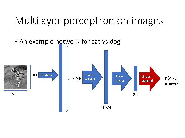
Multilayer perceptron on images • An example network for cat vs dog 256 Reshape 65 K Linear + Re. LU Linear + sigmoid 32 256 1024 p(dog | image)

The linear function • y = Wx + b • How many parameters does a linear function have? dout = din The case when din = 2. A single row in y plotted for every possible value of x

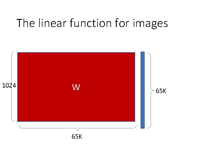
The linear function for images 1024 W 65 K

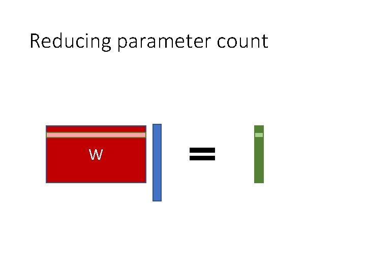
Reducing parameter count W

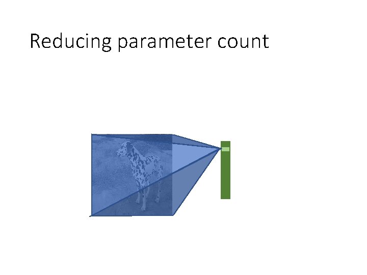
Reducing parameter count

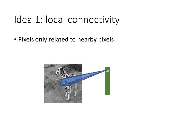
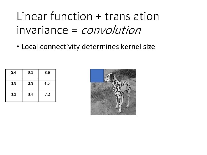
Idea 1: local connectivity • Pixels only related to nearby pixels

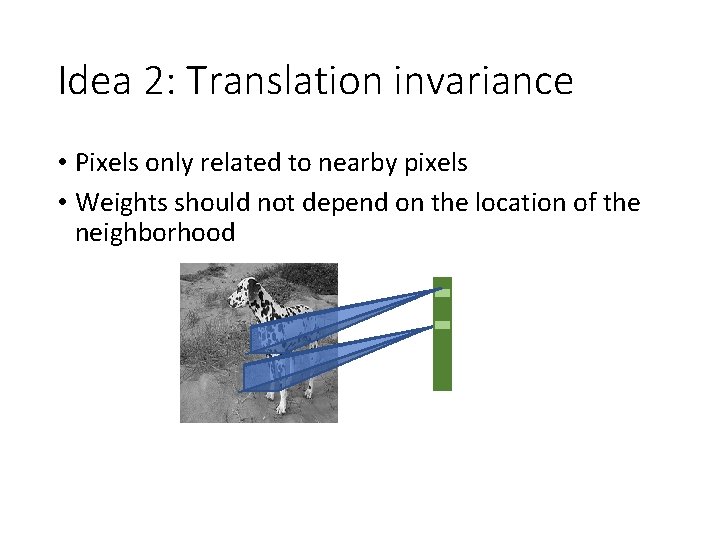
Idea 2: Translation invariance • Pixels only related to nearby pixels • Weights should not depend on the location of the neighborhood

Linear function + translation invariance = convolution • Local connectivity determines kernel size 5. 4 0. 1 3. 6 1. 8 2. 3 4. 5 1. 1 3. 4 7. 2

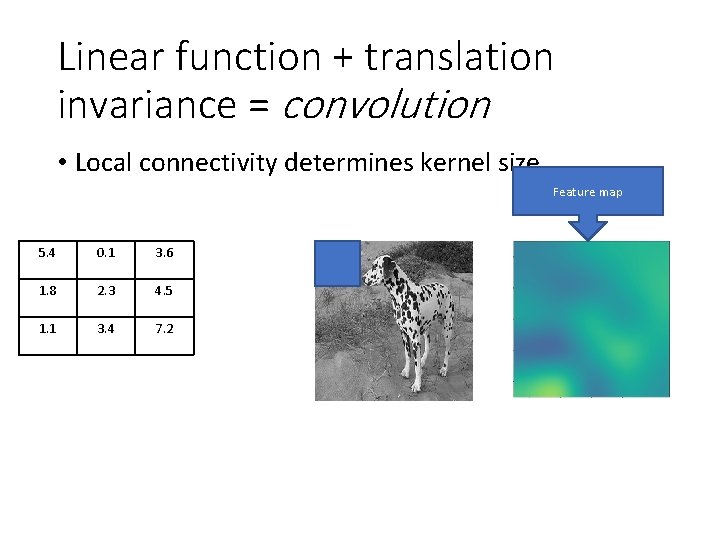
Linear function + translation invariance = convolution • Local connectivity determines kernel size Feature map 5. 4 0. 1 3. 6 1. 8 2. 3 4. 5 1. 1 3. 4 7. 2

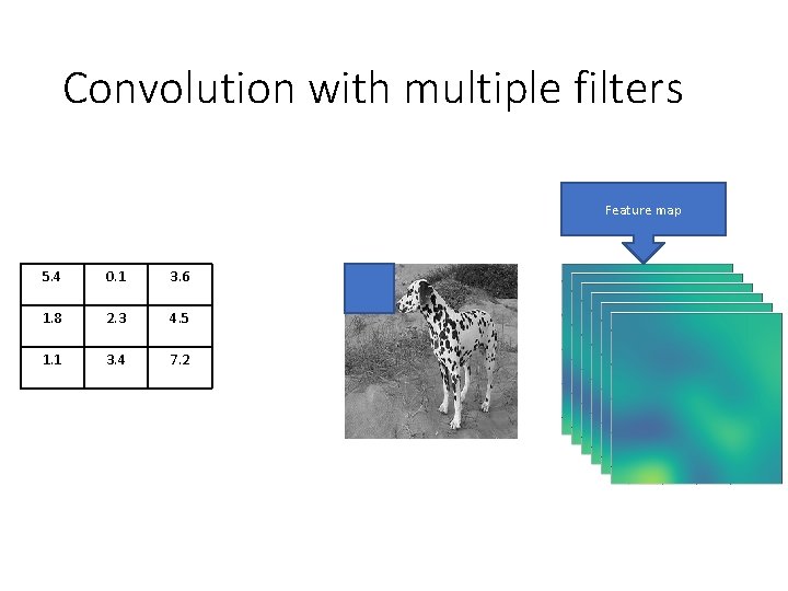
Convolution with multiple filters Feature map 5. 4 0. 1 3. 6 1. 8 2. 3 4. 5 1. 1 3. 4 7. 2

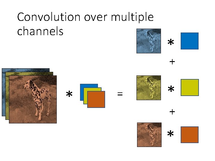
Convolution over multiple channels * + * = * + *

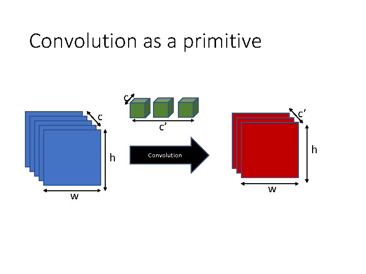
Convolution as a primitive c c c’ h w c’ h Convolution w

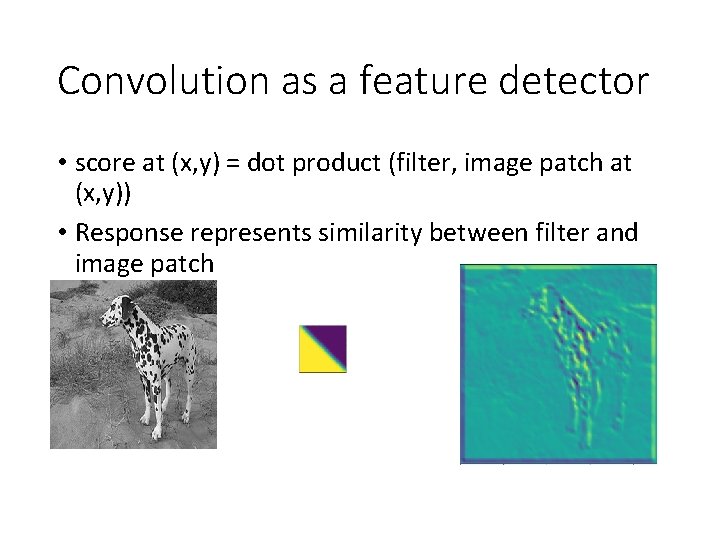
Convolution as a feature detector • score at (x, y) = dot product (filter, image patch at (x, y)) • Response represents similarity between filter and image patch

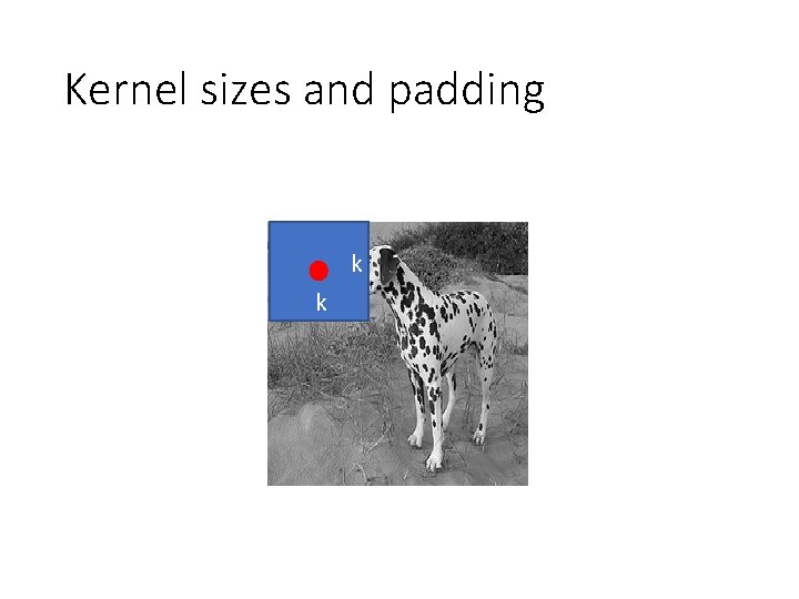
Kernel sizes and padding k k

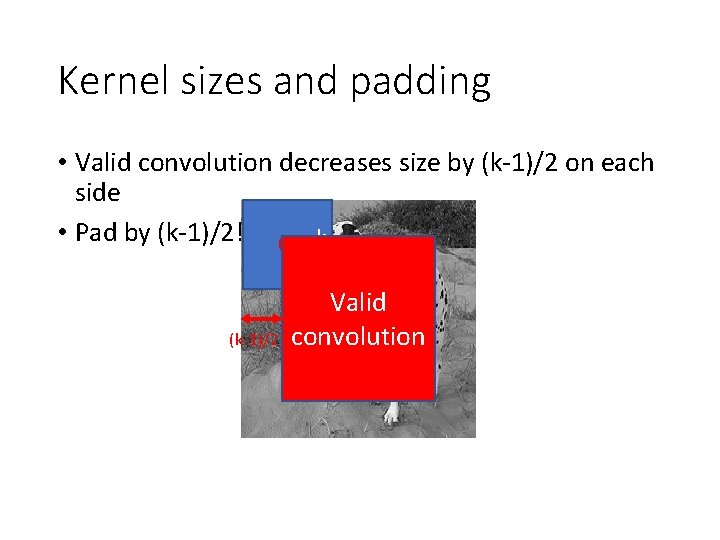
Kernel sizes and padding • Valid convolution decreases size by (k-1)/2 on each side • Pad by (k-1)/2! k k (k-1)/2 Valid convolution

The convolution unit • Each convolutional unit takes a collection of feature maps as input, and produces a collection of feature maps as output • Parameters: Filters (+bias) • If cin input feature maps and cout output feature maps • Each filter is k x cin • There are cout such filters • Other hyperparameters: padding

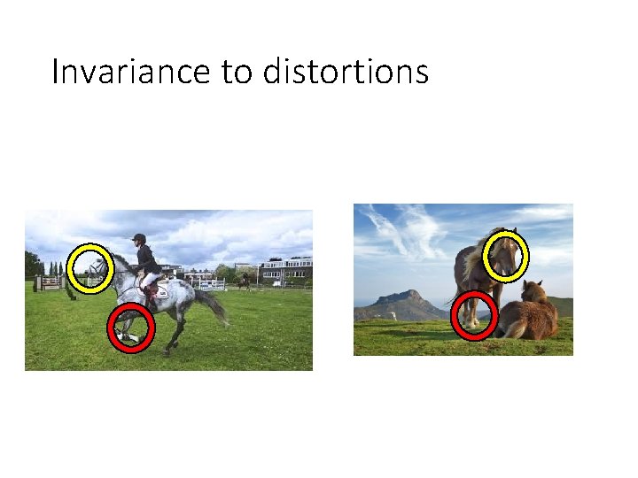
Invariance to distortions

Invariance to distortions

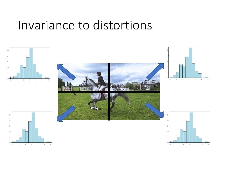
Invariance to distortions

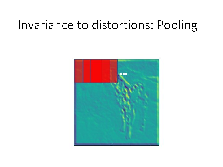
Invariance to distortions: Pooling …

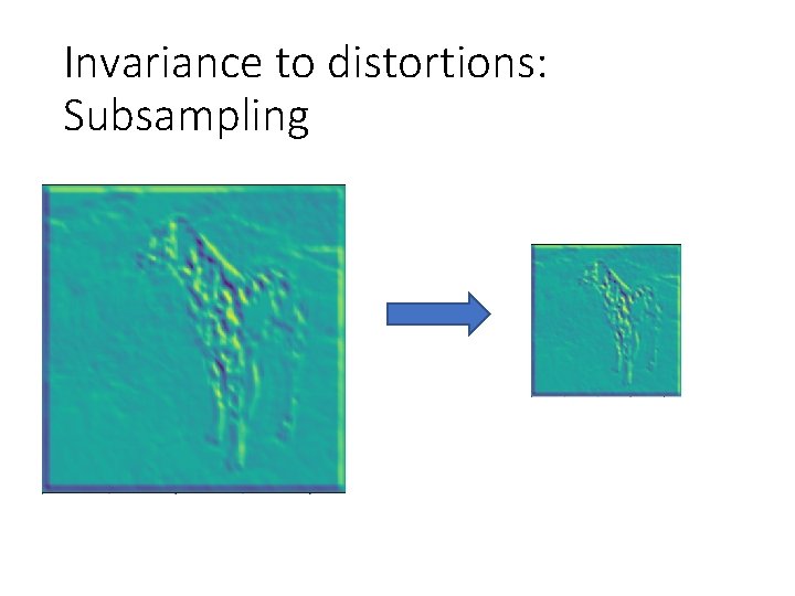
Invariance to distortions: Subsampling

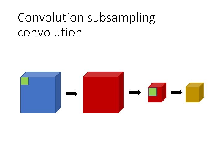
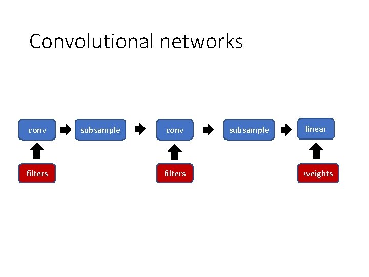
Convolution subsampling convolution

Convolution subsampling convolution • Convolution in earlier steps detects more local patterns less resilient to distortion • Convolution in later steps detects more global patterns more resilient to distortion • Subsampling allows capture of larger, more invariant patterns

Strided convolution • Convolution with stride s = standard convolution + subsampling by picking 1 value every s values • Example: convolution with stride 2 = standard convolution + subsampling by a factor of 2

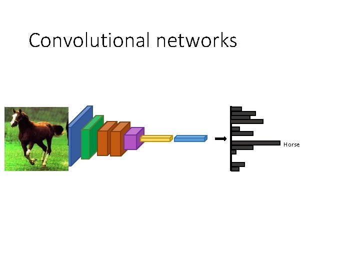
Convolutional networks Horse

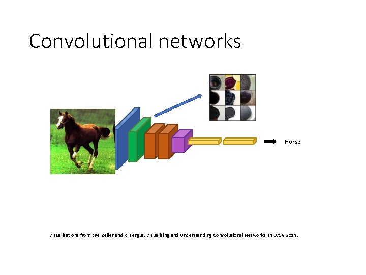
Convolutional networks Horse Visualizations from : M. Zeiler and R. Fergus. Visualizing and Understanding Convolutional Networks. In ECCV 2014.

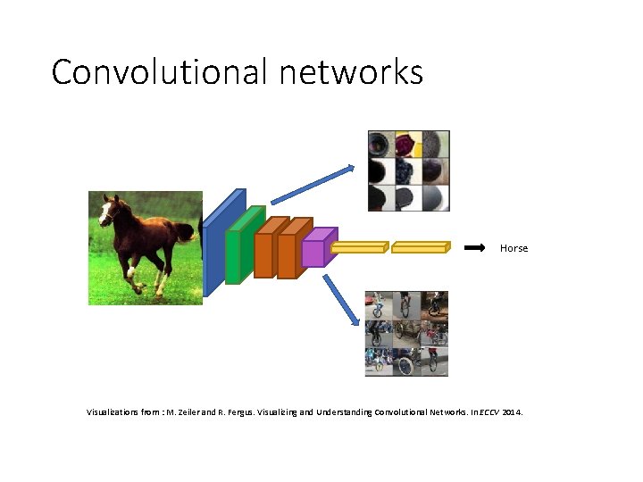
Convolutional networks Horse Visualizations from : M. Zeiler and R. Fergus. Visualizing and Understanding Convolutional Networks. In ECCV 2014.

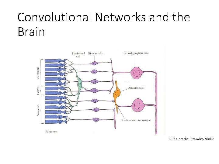
Convolutional Networks and the Brain Slide credit: Jitendra Malik

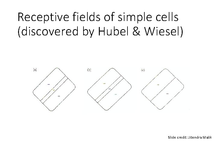
Receptive fields of simple cells (discovered by Hubel & Wiesel) Slide credit: Jitendra Malik

Convolutional networks Yann Le. Cun, Léon Bottou, Yoshua Bengio, and Patrick Haffner. Gradient-based learning applied to document recognition. Proceedings of the IEEE 86. 11 (1998): 2278 -2324.

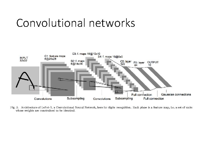
Convolutional networks

Convolutional networks conv filters subsample linear weights