NonLinear Classifiers 2 SVM Pattern Recognition and Image

Non-Linear Classifiers 2: SVM Pattern Recognition and Image Analysis Dr. Manal Helal – Fall 2014 Lecture 10

2 Overview n Kernel Based Methods n RBFs n SVM (Linear recap) n Non Linear SVM n Matlab Examples

3 SVM Pre-requisites n SVM is a kernel based classification method (learning), that depends on some Linear Algebra, Optimisation, and Calculus concepts.

4 Nonlinear Classifiers: Introduction n An example: Suppose we’re in 1 -dimension n What would a linear SVMs do with this data? Positive “plane” Negative “plane”

5 Nonlinear Classifiers: Introduction n Harder 1 -dimensional dataset n What can be done about this?

6 Nonlinear Classifiers: Introduction n non-linear basis function n zk =(xk, xk 2) Positive “plane” Negative “plane”

7 Polynomial Classifier: XOR problem n XOR problem with polynomial function. n With nonlinear polynomial function classes can be classified. n Example XOR-Problem: n linear not separable!

8 Polynomial Classifier: XOR problem With we obtain �(0, 0) (0, 0, 0) �(0, 1) (0, 1, 0) �(1, 0) (1, 0, 0) �(1, 1) (1, 1, 1) . . . that‘s separable in H by the Hyper-plane:

9 Polynomial Classifier: XOR problem n Hyper-plane: �� (�� ) = ���� + �� 0 = 0 is Hyper-plane in H is polynomial in X

10 Polynomial Classifier: XOR problem n Decision Surface in X: Mat. Lab: >> x 1=[-0. 5: 0. 1: 1. 5]; >> x 2=( ). /(2*x 1 -1); >> plot(x 1, x 2);

Polynomial Classifier: XOR problem n With nonlinear polynomial functions, classes can be classified in original space X n Example: XOR-Problem was not linear separable!. . . but linear separable in H !. . . and separable in X with a polynomial function! 11

12 Polynomial Classifier n Decision function is approximated by a polynomial function g(x) , of order p e. g. p=2: n Special case of a Two-Layer Perceptron n Activation function with polynomial input

13 Similarly Map ℝ 2 ℝ 3 (Left) A dataset in ℝ 2 , not linearly separable. (Right) The same dataset transformed to ℝ 3 by the transformation: 2 2 [�� 1, �� 2] [�� 1, �� 2, �� 1 + �� 2 ]

Non-Linear SVM in Higher dimensions n Given a dataset that is not linearly separable in ℝN may be linearly separable in a higher-dimensional space ℝM (where M > N). n Thus, if we have a transformation that lifts the dataset to a higher-dimensional such that is linearly separable, then we can train a linear SVM on to find a decision boundary that separates the classes in ℝM. n Projecting the decision boundary found in back to the original space will yield a nonlinear decision boundary. n Visualisations: n "SVM with polynomial kernel visualization" n "Performing nonlinear classification via linear separation in higher dimensional space" 14

15 What about if M is too large? n

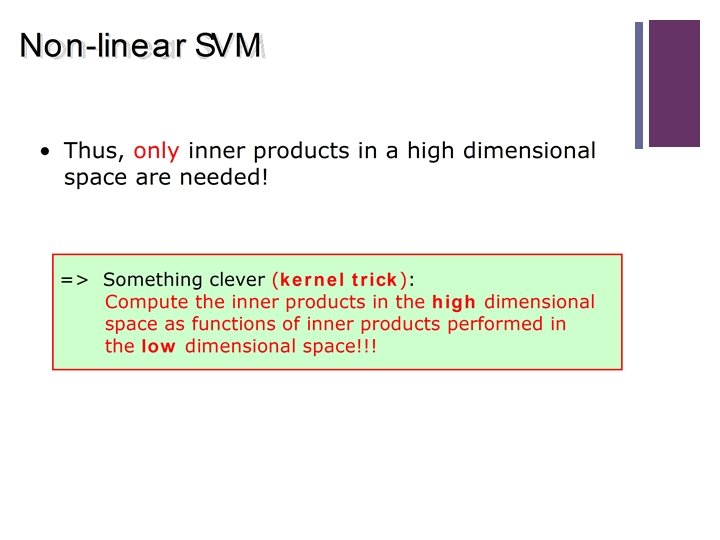
16 The Kernel Trick (We only need dot products) n Give me the numeric result of (�� + �� )10 for some values of �� and ��. n By The Binomial Theorem: 10+10�� 9�� 8�� 2+120�� 7�� 3+210�� 6�� 4+252�� 5+210�� 4�� 6+120�� 3�� 7+45�� 2�� 8+10�� �� +45�� 9+�� 10 �� n The trick: we can evaluate the dot product between degree 10 polynomials without explicitly forming them. Valid kernels are dot products where we can compute the numeric result between two points without having to form their explicit feature values. n �� (��, = <ϕ(�� ), ��) ϕ(�� )> where <. , . > is the inner product in the new space. We don’t even need to know what ϕ is

Representation Theory A portion of the vector field (sin y, sin x) n In vector calculus, a vector field is an assignment of a vector to each point in a subset of space. n A vector space is a mathematical structure formed by a collection of vectors, which may be added together and multiplied ("scaled") by a factor, preserving the group structure n The geometric properties of a family of surfaces in a 3 D Euclidian space, can be studied using the vector fields of the unit normals on these surfaces. n A basis vector is a set of linearly independent vectors that, in a linear combination, can represent every vector in a given vector space or free module, or, more simply put, which define a "coordinate system”. Generally, a basis is a linearly independent spanning set. 17 The same vector can be represented in two different bases (purple and red arrows).

18 Orthogonality explains the trick n It is the relation of two lines at right angles to one another (perpendicularity). n It describes non-overlapping, uncorrelated, or independent objects of some kind. n The dot product of two vectors measures the angle between them. Two vectors are orthogonal, when their dot product is equal to zero. (arccos(0) = 90°).

Example We don’t always have domain experts, and need to predict the model 19

20 Linear Regression n Linear Regression fits the data (n), �� (n)), n = 1, 2, . . N}) D = {(�� n to a linear equation ��(��) = a�� + b, n by choosing the weights T = (a, b)T �� n of the feature map Tϕ(��) ��(��) = �� n that minimize the squared prediction error Tϕ(n)(�� (n)) ]2 E (��)n[�� =(n)Σ = ��

21 Linear Regression in Matrix Form n In matrix form the Error Function is: T(�� T –�� Tϕ) E(��)T =–�� ϕ)T (�� (n) and ϕ = ϕ (�� with �� n = �� ij i j) n Minimum Error is obtained by: -1ϕ�� �� =T)(�� where (ϕϕT)-1ϕ is called the Moore-Penrose pseudo inverse of ϕ (ϕϕT) is an Mx. M matrix where M is the number of basis functions O(M 3) operations to calculate (ϕϕT)-1ϕ

22 Dealing with unknown Basis Functions n One way to deal with over-fitting is by using regularization. n However, it will not help much if the basis functions do not match the data. n So, what we should do if we do not know the model? n Is there a universal set of basis functions that can approximate arbitrary functions reasonably well?

23 More Complex Basis functions n We can also use more complex mode, for example a 3 rd degree polynomial : n 2++�� 3. ��(��) = 3�� �� �� 1 + �� 2�� 4�� n This yields the feature map: 1 ϕ(��) �� = 2 �� 3 �� Quality of Solution? Worse Model Complexity? Higher Why? Model does not match data

24 Linear Regression Using “bump” Functions n Approximate the function with a sum of bump shaped functions

25 Linear Regression Using Radial Basis Functions (RBFs) n Gaussian Radial Basis Functions : The centre is at m(i) and αdetermines the width of the bump. n Advantage: They decrease smoothly to zero and do not show oscillatory behaviour unlike the higher order polynomials.

26 Gaussian RBF in 2 D space

27 Linear Regression using RBFs n Use with i = 1, … 16 as basis functions. Apply linear regression. n In one dimension, this seems to work well, but does it scale to higher dimensions? Approximation of sin(10 x) by 16 Gaussian RBFs. Black Line: Original function Red Line: Regression.

28 Curse of Dimensionality n n To cover the data with a constant discretisation level (number of RBFs per unit volume) the number of basis functions and weights will grows exponentially with the number of dimensions: Dimensions # of basis functions / weights 1 16 2 162 = 256 3 163 = 4096 4 164 = 65536 5 165 = 1048576 : : 10 1610 ≈ 1012 Is there a way to reduce the number of required weights?

29 Dual Representation n Orthogonal Complement Let �� be a subspace. N. of ℝ n ⊥ of �� is the The orthogonal complement �� set of all vectors that are orthogonal to all elements of ��, ⊥ = {z∈ n �� = {c 1(1, 0, 0) + c 2(1, 1, 0), c ∈ ℝ 2} n Tz = 0 ∀ �� ∈�� } ℝN: �� ⊥= {c(0, 0, 1), c ∈ ℝ} �� Orthogonal decomposition n �� N∈can ℝ be written uniquely in the form ŷ = �� + z with ŷ ∈ �� and ⊥z ∈�� �� = (2, 3, 5) ŷ = (2, 3, 0) z = (0, 0, 5)

Null Space of Training Set n Let ��(n)=, {�� n = 1, 2, … N} be the set of all training points n Consider the predictions of the model T�� = �� �� (��) On the training set, i. e. ��∈�� n Using orthogonal decomposition we write, w=ŵ+z with ŵ ∈span(��) and ⊥ z ∈�� n. The prediction becomes: Why this is zero? ��(��) T=�� (ŵ T+=�� z) ŵ T�� + z T=�� ŵ n. Hence, we can assume that �� ∈span(��) 30

31 Dual Representation n The weight vector w is thus a linear combination of the training samples ��. n The parameters �� 1, =…(�� �� N) are called the dual parameters n This also applies when using basis functions, n There as many dual parameters as training samples. Their number is independent of the number of basis functions.

32 Predictions in Dual Representation n Tϕ(��) Substituting w back into the linear regression y(��) = �� yields n With the kernel function ϕ, Gram matrix of a set of vectors v , …, v in an 1 n �� (��, T ��) ϕ(��): = �(��)inner product space is the Hermitian matrix of inner products, whose entries are given by Gij=< n Using the Gram Matrix: vj, vi>. For a Finite Dimensions in Euclidian space, it is G = VTV. It is the avaluation of the kernel (m), (�� (n)) = ϕ(�� (m)) T ϕ(x(n)) function over all pairs of points in the training set. �� : = �� �� mn n (n)) (�� The predictions Yn = �� on the training set are simply YT = a. T��

33 Solution of Dual Representation Primal Representation (Standard Linear Regression) Dual Representation where ϕ is the matrix of feature vectors where �� is the gram matrix (also called the kernel matrix) n. Solution A =(ϕϕT)-1ϕ�� = ϕ+�� T)-1���� +�� A =(���� = �� n. Complexity is O(M 3), where M is the number of basis functions n. Complexity is O(N 3), where N is the number training samples n. Predictions: Tϕ(�� �� (�� ) = �� ) “Components an weighted with (n)” similarity to training sample ��

34 Why is Dual Representation Useful n N is the number of Training Sample n Lots of basis functions & moderate number of training samples: dual representation saves lots of parameters

35 Example: Kernel of RBF n Gaussian RBF basis function: For i = 1, … M n Calculate Kernel: ��(��, T��) ϕ(��) : = =�(��) n Linear Regression: where N is the number of training samples.

36 Example: Kernel of Polynomial Basis n The polynomial basis of order D: i-1, = �� ϕi(��) n i = 1, … , D This expensive ddimensional scalar product is simplified to this geometric series Induces the kernel: �� (��, T ��) ϕ(y) = : = �(��) n And the Gram Matrix: (n) (�� (m)) = �� nm : = ��, �� Evaluating the Kernel is much cheaper than calculating the mapping ϕ into feature space and the scalar product explicitly.

37 Properties of the Kernel n Calculate ϕTϕ componentwise: (ϕTϕ)mn = n Thus we have: Tϕ ��=� with �� symmetric n T���� �� is positive semi-definite, that is ≥ 0 �� for any ��, since 0≤ for any ��

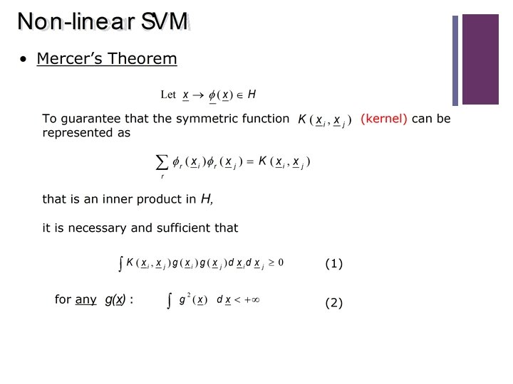
When is a function a Kernel? n Mercer’s theorem (for finite input space): Consider a finite input (N)} with ��(�� (n), �� (m) ) a function on ��. space ��(1)=, …, {�� �� n (n), �� (m) ) is a kernel function, that is a scalar product in a feature Then ��(�� space, if and only if, �� is symmetric and the matrix (n), �� (m) ) is positive semi-definite. �� nm = ��(�� n Proof: 38 �� is symmetric the eigenvalue decomposition has the form �� = TV�V , where Ʌ is a diagonal matrix containing the eigenvalues λt = Ʌtt of �� and V is an orthogonal matrix containing the eigenvectors Vt. �� is positive semi-definite All eigenvalues are non-negative, λt ≥ 0. Define the feature map: And see if it corresponds to the kernel by calculating the scalar product :

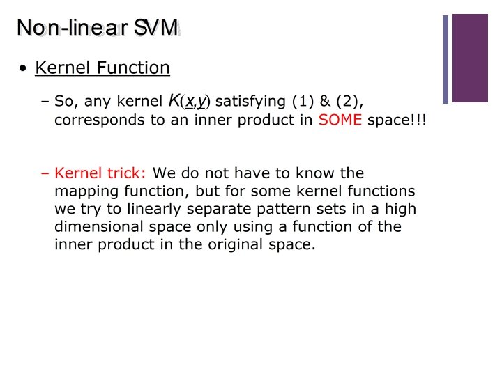
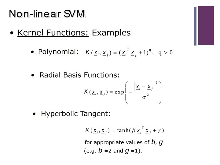
39 Kernels Summary n Kernels compute the value of a scalar product in high dimensional feature space without explicitly computing the features. n They can be used in any model that depends (or can be rewritten so that it depends) on the scalar product of the training samples. n Not every function is a kernel. n Use Kernel construction rules to prove that a function is a valid kernel.

40

Math Review: Hyper-planes in Hessian Normal Form n 41 For a point �� 1 that lies on the far side of the hyper-plane we have: T�� �� 1 + �� > 0 Because the projection of �� 1 on �� is larger than for points �� that ar the hyper-plane. n Conversely for a point �� 2 that lies on the near side of the hyperplane, we have, T�� �� 2 + �� < 0 Because the projection of �� 2 on �� is smaller than for points �� that are on the hyper-plane. n T�� Linear Classifier h(��) = �� + b is classified by checking the sign(h(��) ).

Linear Classifier with a Margin n We add two more hyper-planes that are parallel to the original hyper-plane and require that no training point must lie on between those hyper-planes. n Thus we now require: T�� + (�� - ��) > blue �� 0 forclass �� from And the T�� + (�� + ��) < 0 �� for green allclass. �� from the The distance from the origin to the T�� + �� = 0 is given by: hyper-plane �� d= -��/|��|, thus dblue = -(��-��)/|��| dgreen = -(��+��)/|��| And the margin is m= dblue - dgreen= 2��/|��| ≈ 2/|��| 42

43 Set of Constraints n n th Let �� -1, 1} the class assigned to �� i be the i data, and �� i ∈ { i. The constraints are: : T�� �� i + �� ≥ +1 for �� i = +1 T�� �� i + �� ≤ -1 for �� i = -1 Can be condensed to: T�� �� 1 all i. i(�� i + ��) ≥for n If these constraints are fulfilled, the margin is:

44 Optimisation Problem n th Let �� -1, 1} the class assigned i be the i data, i = 1, … m, and �� i ∈ { to �� i. To find the separating hyper-plane with the maximum margin we: T�� minimise �� ) =½ �� 0 (��, �� T�� subject to: �� �� )i +=��) – 1 ≥ 0 for i i (��, �� i(�� = 1, . . . , m n This is a constrained convex optimisation problem. n Note that we introduced the arbitrary ½ in the objective function �� 0 (��, �� ) to obtain nicer derivative later on.

Dual Problem n We apply the recipe for solving the constrained optimisation problem. n 1. Calculate the Lagrangian: n n L(��, �� T�� , α) -= ½�� 2. Minimise L(��, �� , α) w. r. t �� and �� Thus the weights are a linear combination of the training samples: 45

46 Dual Problem n Substituting both relations back to L(��, �� , α) gives us the Lagran dual function �� (α). Thus: Maximise �� (α) = Subject to αi ≥ 0 i=1, … m We will demonstrate the an efficient algorithm to solve the dual problem. The bias �� does not appear in the dual problem and thus needs to be recovered afterwards. But for both issues we need to derive some properties of the solution first.

Support Vectors n Remember that the optimal solution must satisfy amongst others the KKT complimentary slackness condition: *)=0 αi�� i(�� n In our case, this means: T�� αi[�� for all i i(�� i + ��) – 1] =0 n Hence, a training sample �� i can only contribute to the weight vector (αi≠ 0) if it lies on the margin, that is T�� �� i(�� i + ��) = 1 n a training sample �� i with (αi≠ 0) is called a support vector n T�� The class of �� is h(��) = sign(�� + ��), substitutinggives: n We only need to remember the few training samples where (αi≠ 0). 47

48 Recovering the bias n From the complimentary slackness condition αi�� i(��)=0, we can recover the bias. n When we take the support vector (αi≠ 0), the corresponding constraint �� i (��, �� ) must be zero and thus we have: T�� �� i + �� i = �� n Solving this for �� gives the bias: ��i - �� =T�� i �� where n . We can use any support vector to calculate the bias.

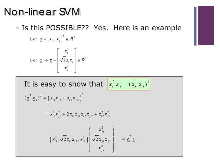
49 Non Linear SVM: The XOR Problem n Linear separation in high dimensional space H via nonlinear functions (polynomial and RBF’s) in the original space X. n For this we found nonlinear mappings ϕ(�� ): X H Is that possible without knowing the mapping function � ? !?

Non-linear Support Vector Machines n Recall that, the probability of having linearly separable classes increases as the dimensionality of feature vectors increases. n Assume the mapping: �� �Rl �z �Rk, k �l n Then use linear SVM in Rk n Recall that in this case the dual problem formulation will be : n The classifier will be: 50

Non-linear SVM Formulation 56

57 Linear SVM – Pol SVM in the input Space X

58 Pol. SVM – RBF SVM in the input space X

59 Pol. SVM – RBF SVM in the input space X

60 SVM vs. Neural Networks n Training a Support Vector Machine (SVM) involves optimization of a concave function: there is a unique solution n Training a neural network learning model is generally nonconvex: there are potentially different solutions depending on the starting values for the model parameters.

61 SVM Software

Matlab SVM Functions n 62 For the exam dataset, the polynomial kernel function in SVM was the best scoring: xtrain = Dataset(1: 80, 1: 2) ytrain = Dataset(1: 80, 3) xtest = Dataset(81: 100, 1: 2) %The Polynomial Kernel SVM classifier: SVMStruct = svmtrain(xtrain, ytrain, 'kernel_function', 'polynomial’) ytest = svmclassify(SVMStruct , xtest ) bad = ~strcmp(svmclassify(SVMStruct , xtrain), ytrain) P_SVMResub. Err = sum(bad) / 80 cp = cvpartition(ytrain, 'k', 10) SVMClass. Fun = @(xtrain, ytrain, xtest (svmclassify(SVMStruct , xtest)) P_SVMCVErr = crossval('mcr', xtrain, ytrain, 'predfun', SVMClass. Fun, 'partition', cp)

63 Other Matlab SVM functions SVMModel 1 = fitcsvm(xtrain, ytrain, 'Kernel. Function', 'polynomial', 'Standardize', true); % Compute the scores over a grid d = 0. 02; % Step size of the grid [x 1 Grid, x 2 Grid] = meshgrid(min(xtrain(: , 1)): d: max(xtrain(: , 1)), . . . min(xtrain(: , 2)): d: max(xtrain(: , 2))); x. Grid = [x 1 Grid(: ), x 2 Grid(: )]; % The grid [~, scores 1] = predict(SVMModel 1, x. Grid); % The scores figure; h(1: 2) = gscatter(xtrain(: , 1), xtrain(: , 2), ytrain) hold on h(3) = plot(xtrain(SVMModel 1. Is. Support. Vector, 1), . . . xtrain(SVMModel 1. Is. Support. Vector, 2), 'ko', 'Marker. Size', 10); % Support vectors contour(x 1 Grid, x 2 Grid, reshape(scores 1(: , 2), size(x 1 Grid)), [0 0], 'k'); % Decision boundary title('Scatter Diagram with the Decision Boundary') legend({'-1', 'Support Vectors'}, 'Location', 'Best'); hold off