NonExperimental designs Psych 231 Research Methods in Psychology

Non-Experimental designs Psych 231: Research Methods in Psychology

n Don’t forget Quiz 8 is due on Apr. 9 th at midnight n Post Exam 2 extra credit – posted on Reggie. Net, due in -class on Tuesday (4/5) n New extra-credit option – ISU research symposia/poster session (This Friday) – Use the same questions as the research participation, 2 posters = 1/2 hour study = 1 journal summary writeup Reminders

n Sometimes you just can’t perform a fully controlled experiment n n Because of the issue of interest Limited resources (not enough subjects, observations are too costly, etc). • Surveys • Correlational • Quasi-Experiments • Developmental designs • Small-N designs n This does NOT imply that they are bad designs n Just remember the advantages and disadvantages of each Non-Experimental designs

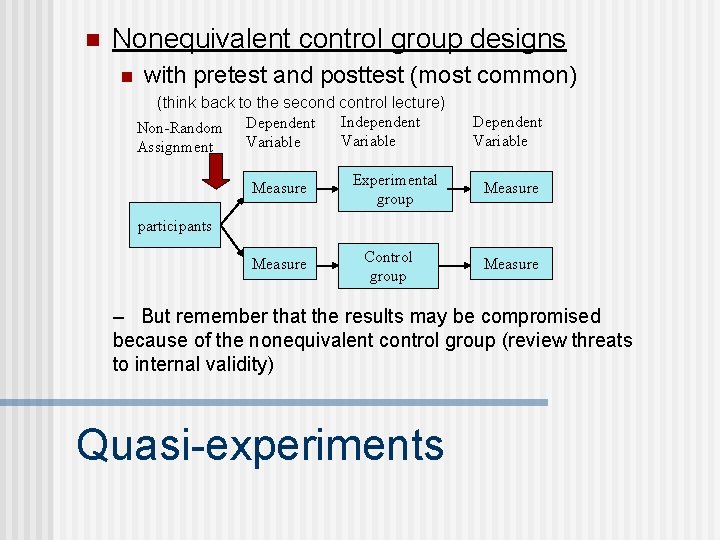
n Nonequivalent control group designs n with pretest and posttest (most common) (think back to the second control lecture) Independent Non-Random Dependent Variable Assignment Measure Experimental group Dependent Variable Measure participants Measure Control group Measure – But remember that the results may be compromised because of the nonequivalent control group (review threats to internal validity) Quasi-experiments

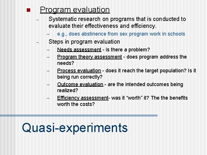
Program evaluation n – Systematic research on programs that is conducted to evaluate their effectiveness and efficiency. – – e. g. , does abstinence from sex program work in schools Steps in program evaluation – – – Needs assessment - is there a problem? Program theory assessment - does program address the needs? Process evaluation - does it reach the target population? Is it being run correctly? Outcome evaluation - are the intended outcomes being realized? Efficiency assessment- was it “worth” it? The the benefits worth the costs? Quasi-experiments

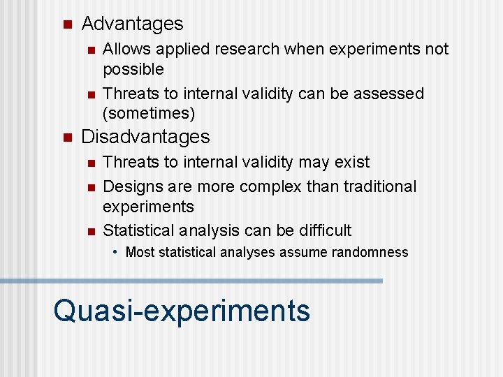
n Advantages n n n Allows applied research when experiments not possible Threats to internal validity can be assessed (sometimes) Disadvantages n n n Threats to internal validity may exist Designs are more complex than traditional experiments Statistical analysis can be difficult • Most statistical analyses assume randomness Quasi-experiments

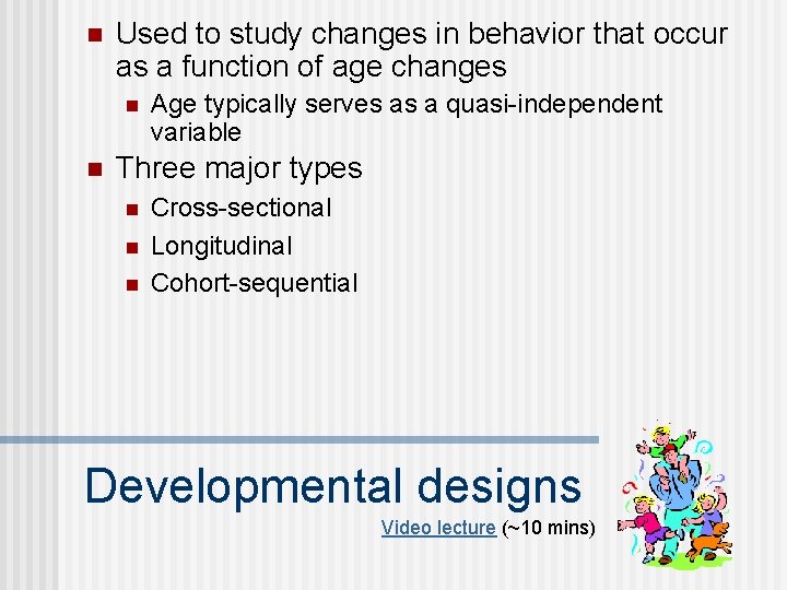
n Used to study changes in behavior that occur as a function of age changes n n Age typically serves as a quasi-independent variable Three major types n n n Cross-sectional Longitudinal Cohort-sequential Developmental designs Video lecture (~10 mins)

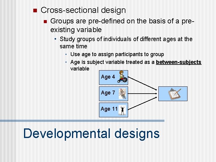
n Cross-sectional design n Groups are pre-defined on the basis of a preexisting variable • Study groups of individuals of different ages at the same time • Use age to assign participants to group • Age is subject variable treated as a between-subjects variable Age 4 Age 7 Age 11 Developmental designs

n Cross-sectional design n Advantages: • • Can gather data about different groups (i. e. , ages) at the same time Participants are not required to commit for an extended period of time Developmental designs

n Cross-sectional design n Disavantages: • Individuals are not followed over time • Cohort (or generation) effect: individuals of different ages may be inherently different due to factors in the environment • • • Are 5 year old different from 15 year olds just because of age, or can factors present in their environment contribute to the differences? • Imagine a 15 yr old saying “back when I was 5 I didn’t have a Wii, my own cell phone, or a netbook” Does not reveal development of any particular individuals Cannot infer causality due to lack of control Developmental designs

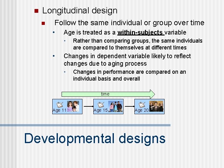
n Longitudinal design n Follow the same individual or group over time • Age is treated as a within-subjects variable • • Rather than comparing groups, the same individuals are compared to themselves at different times Changes in dependent variable likely to reflect changes due to aging process • Changes in performance are compared on an individual basis and overall time Age 11 Age 15 Age 20 Developmental designs

n Examples n Wisconsin Longitudinal Study (WLS) • Began in 1957 and is still on-going (50 years) • 10, 317 men and women who graduated from Wisconsin high schools in 1957 • Originally studied plans for college after graduation • Now it can be used as a test of aging and maturation • Data collected in: • 1957, 1964, 1975, 1992, 2004, 2011 n n Physicians’ Health Study Nurses’ Health Study Longitudinal Designs

n Longitudinal design n Advantages: • Can see developmental changes clearly • Can measure differences within individuals • Avoid some cohort effects (participants are all from same generation, so changes are more likely to be due to aging) Developmental designs

n Longitudinal design n Disadvantages • Can be very time-consuming • Can have cross-generational effects: n n Baby boomers Generation X Mellennials Generation Z • Conclusions based on members of one generation may not apply to other generations • Numerous threats to internal validity: • Attrition/mortality • History • Practice effects • Improved performance over multiple tests may be due to practice taking the test • Cannot determine causality Developmental designs

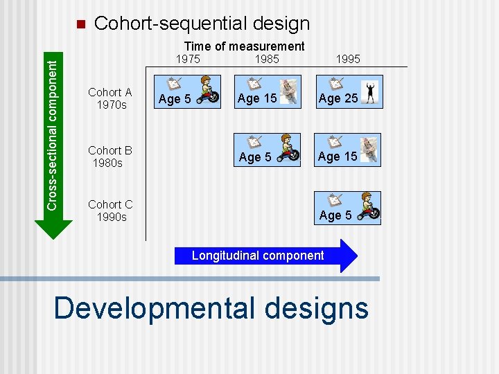
n Cohort-sequential design n Measure groups of participants as they age • Example: measure a group of 5 year olds, then the same group 10 years later, as well as another group of 5 year olds n Age is both between and within subjects variable • Combines elements of cross-sectional and longitudinal designs • Addresses some of the concerns raised by other designs • For example, allows to evaluate the contribution of cohort effects Developmental designs

n Cohort-sequential design Cross-sectional component Time of measurement 1975 Cohort A 1970 s Cohort B 1980 s Cohort C 1990 s Age 5 1985 1995 Age 15 Age 25 Age 15 Age 5 Longitudinal component Developmental designs

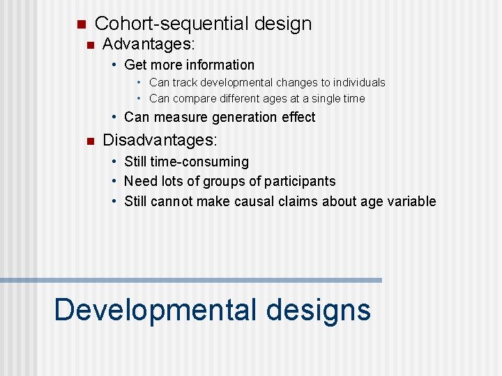
n Cohort-sequential design n Advantages: • Get more information • Can track developmental changes to individuals • Can compare different ages at a single time • Can measure generation effect n Disadvantages: • Still time-consuming • Need lots of groups of participants • Still cannot make causal claims about age variable Developmental designs

n Sometimes you just can’t perform a fully controlled experiment n n Because of the issue of interest Limited resources (not enough subjects, observations are too costly, etc). • Surveys • Correlational • Quasi-Experiments • Developmental designs • Small-N designs n This does NOT imply that they are bad designs n Just remember the advantages and disadvantages of each Non-Experimental designs

n What are they? n In contrast to Large N-designs (comparing aggregated performance of large groups of participants) • One or a few participants • Data are typically not analyzed statistically; rather rely on visual interpretation of the data n Historically, these were the typical kind of design used until 1920’s when there was a shift to using larger sample sizes • Even today, in some sub-areas, using small N designs is common place • (e. g. , psychophysics, clinical settings, animal studies, expertise, etc. ) Small N designs

n Small vs. Large N debate n Some researchers have argued that Small N designs are the best way to go. • The goal of psychology is to describe behavior of an individual • Looking at data collapsed over groups “looks” in the wrong place • Need to look at the data at the level of the individual Small N designs

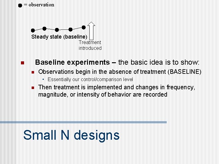
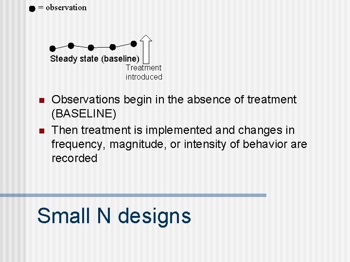
= observation Steady state (baseline) Treatment introduced Baseline experiments – the basic idea is to show: n n Observations begin in the absence of treatment (BASELINE) • Essentially our control/comparison level n Then treatment is implemented and changes in frequency, magnitude, or intensity of behavior are recorded Small N designs

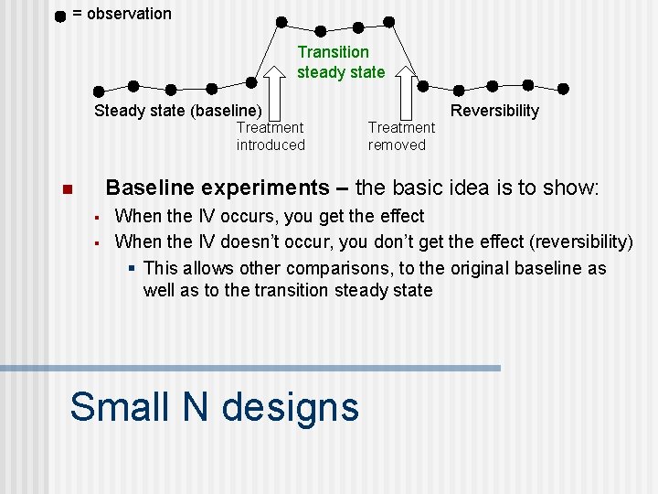
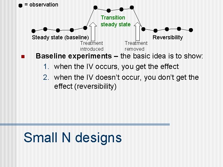
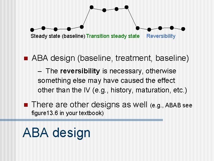
= observation Transition steady state Steady state (baseline) Treatment introduced Treatment removed Reversibility Baseline experiments – the basic idea is to show: n § § When the IV occurs, you get the effect When the IV doesn’t occur, you don’t get the effect (reversibility) § This allows other comparisons, to the original baseline as well as to the transition steady state Small N designs

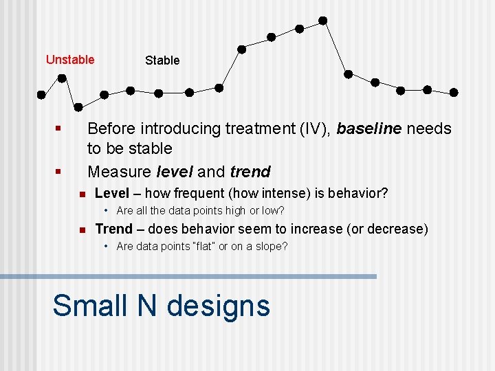
Unstable § Stable Before introducing treatment (IV), baseline needs to be stable Measure level and trend § n Level – how frequent (how intense) is behavior? • Are all the data points high or low? n Trend – does behavior seem to increase (or decrease) • Are data points “flat” or on a slope? Small N designs

Steady state (baseline) Transition steady state n Reversibility ABA design (baseline, treatment, baseline) – The reversibility is necessary, otherwise something else may have caused the effect other than the IV (e. g. , history, maturation, etc. ) n There are other designs as well (e. g. , ABAB see figure 13. 6 in your textbook) ABA design

n Advantages n n n Focus on individual performance, not fooled by group averaging effects Focus is on big effects (small effects typically can’t be seen without using large groups) Avoid some ethical problems – e. g. , with nontreatments Allows to look at unusual (and rare) types of subjects (e. g. , case studies of amnesics, experts vs. novices) Often used to supplement large N studies, with more observations on fewer subjects Small N designs

n Disadvantages n n n Difficult to determine how generalizable the effects are Effects may be small relative to variability of situation so NEED more observation Some effects are by definition between subjects • Treatment leads to a lasting change, so you don’t get reversals Small N designs

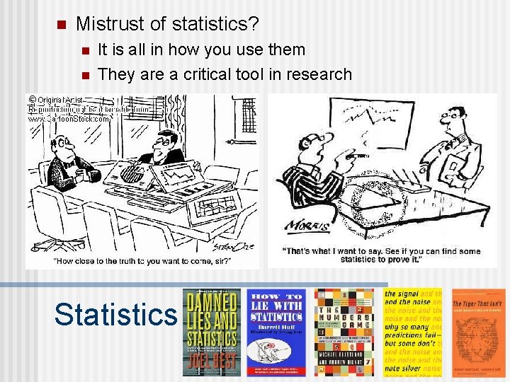
n Mistrust of statistics? n n It is all in how you use them They are a critical tool in research Statistics

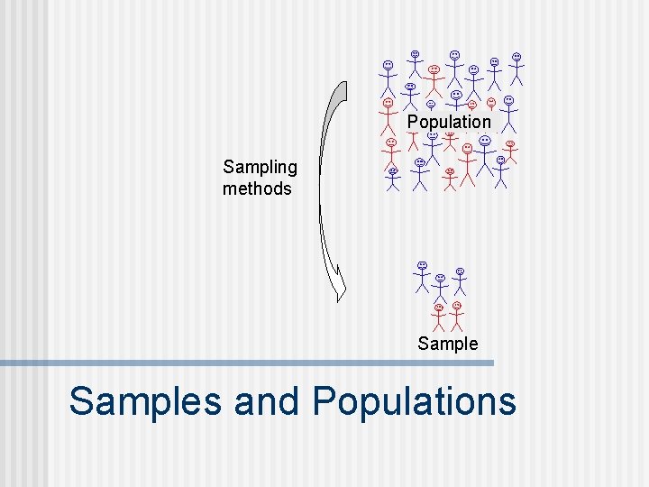
Population Sampling methods Samples and Populations

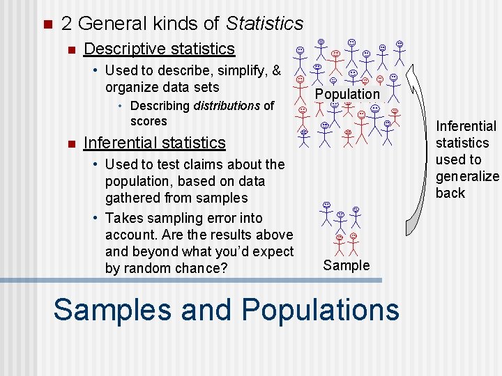
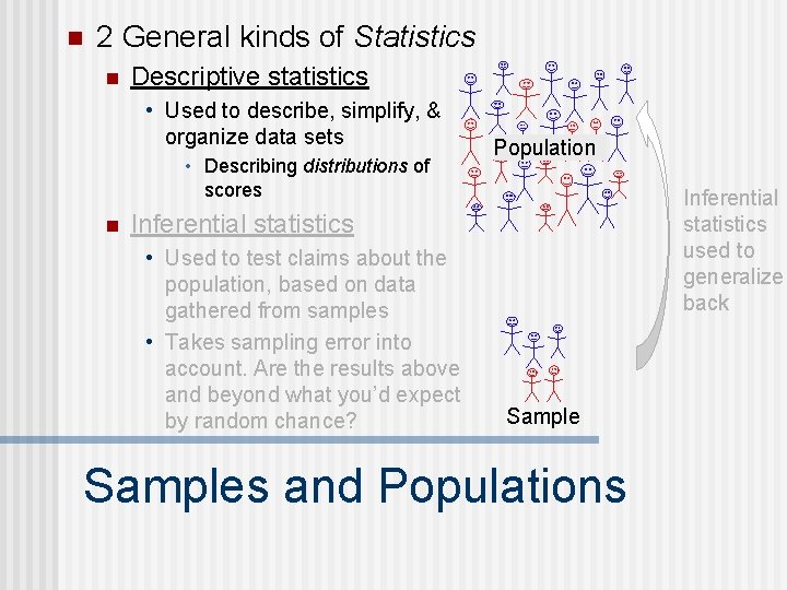
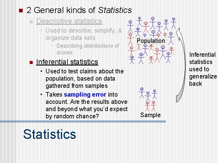
n 2 General kinds of Statistics n Descriptive statistics • Used to describe, simplify, & organize data sets • Describing distributions of scores n Population Inferential statistics used to generalize back Inferential statistics • Used to test claims about the population, based on data gathered from samples • Takes sampling error into account. Are the results above and beyond what you’d expect by random chance? Samples and Populations

n 2 General kinds of Statistics n Descriptive statistics • Used to describe, simplify, & organize data sets • Describing distributions of scores n Population Inferential statistics used to generalize back Inferential statistics • Used to test claims about the population, based on data gathered from samples • Takes sampling error into account. Are the results above and beyond what you’d expect by random chance? Samples and Populations

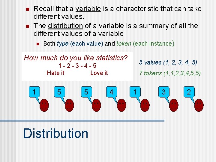
n n Recall that a variable is a characteristic that can take different values. The distribution of a variable is a summary of all the different values of a variable n Both type (each value) and token (each instance) How much do you like statistics? 5 values (1, 2, 3, 4, 5) 1 -2 -3 -4 -5 Hate it Love it 1 5 5 Distribution 7 tokens (1, 1, 2, 3, 4, 5, 5) 4 1 3 2

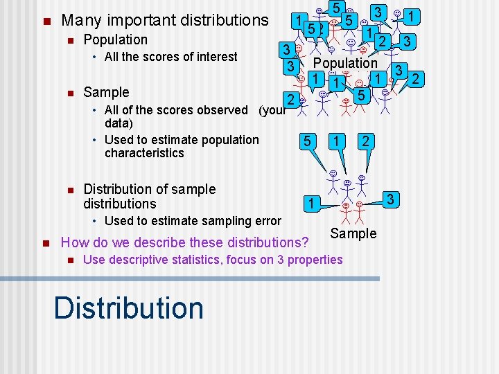
n Many important distributions n Population • All the scores of interest n 1 Sample Distribution of sample distributions 52 3 3 • All of the scores observed (your data) • Used to estimate population characteristics n 5 2 5 1 2 3 Sample Use descriptive statistics, focus on 3 properties Distribution 1 1 How do we describe these distributions? n 3 Population 3 1 1 1 2 5 • Used to estimate sampling error n 5

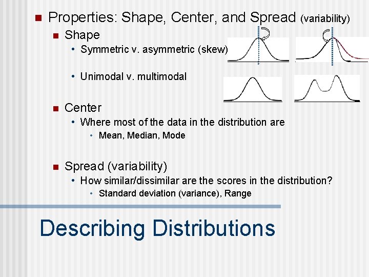
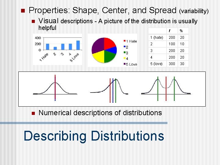
n Properties: Shape, Center, and Spread (variability) n Shape • Symmetric v. asymmetric (skew) • Unimodal v. multimodal n Center • Where most of the data in the distribution are • Mean, Median, Mode n Spread (variability) • How similar/dissimilar are the scores in the distribution? • Standard deviation (variance), Range Describing Distributions

n Properties: Shape, Center, and Spread (variability) n Visual descriptions - A picture of the distribution is usually helpful n f % 1 (hate) 200 20 2 100 10 3 200 20 4 200 20 5 (love) 300 30 Numerical descriptions of distributions Describing Distributions

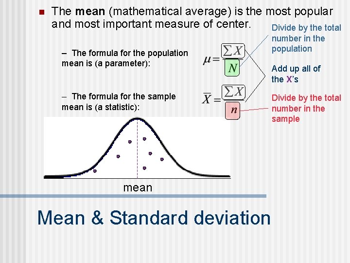
n The mean (mathematical average) is the most popular and most important measure of center. Divide by the total – The formula for the population mean is (a parameter): – The formula for the sample mean is (a statistic): mean Mean & Standard deviation number in the population Add up all of the X’s Divide by the total number in the sample

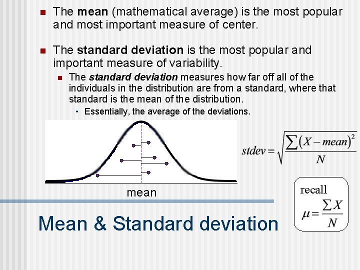
n The mean (mathematical average) is the most popular and most important measure of center. n The standard deviation is the most popular and important measure of variability. n The standard deviation measures how far off all of the individuals in the distribution are from a standard, where that standard is the mean of the distribution. • Essentially, the average of the deviations. mean Mean & Standard deviation recall

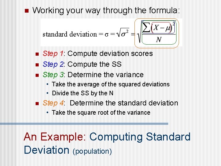
n Working your way through the formula: standard deviation = σ = n n n Step 1: Compute deviation scores Step 2: Compute the SS Step 3: Determine the variance • Take the average of the squared deviations • Divide the SS by the N n Step 4: Determine the standard deviation • Take the square root of the variance An Example: Computing Standard Deviation (population)

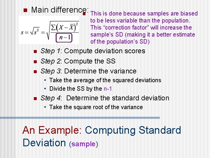
n Main difference: n This is done because samples are biased to be less variable than the population. This “correction factor” will increase the sample’s SD (making it a better estimate of the population’s SD) n n n Step 1: Compute deviation scores Step 2: Compute the SS Step 3: Determine the variance • Take the average of the squared deviations • Divide the SS by the n-1 n Step 4: Determine the standard deviation • Take the square root of the variance An Example: Computing Standard Deviation (sample)

n 2 General kinds of Statistics n Descriptive statistics • Used to describe, simplify, & organize data sets • Describing distributions of scores n Population Inferential statistics used to generalize back Inferential statistics • Used to test claims about the population, based on data gathered from samples • Takes sampling error into account. Are the results above and beyond what you’d expect by random chance? Statistics Sample

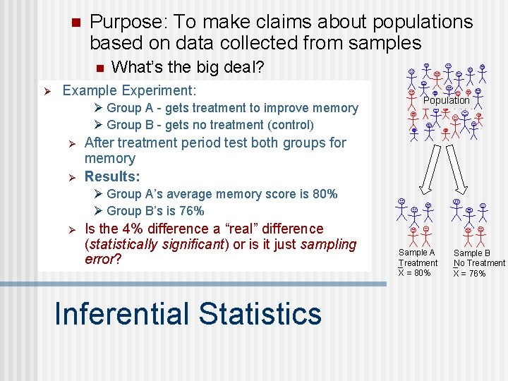
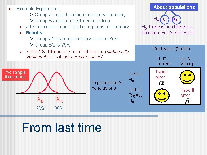
n Purpose: To make claims about populations based on data collected from samples n Ø What’s the big deal? Example Experiment: Ø Group A - gets treatment to improve memory Ø Group B - gets no treatment (control) Ø Ø Population After treatment period test both groups for memory Results: Ø Group A’s average memory score is 80% Ø Group B’s is 76% Ø Is the 4% difference a “real” difference (statistically significant) or is it just sampling error? Inferential Statistics Sample A Treatment X = 80% Sample B No Treatment X = 76%

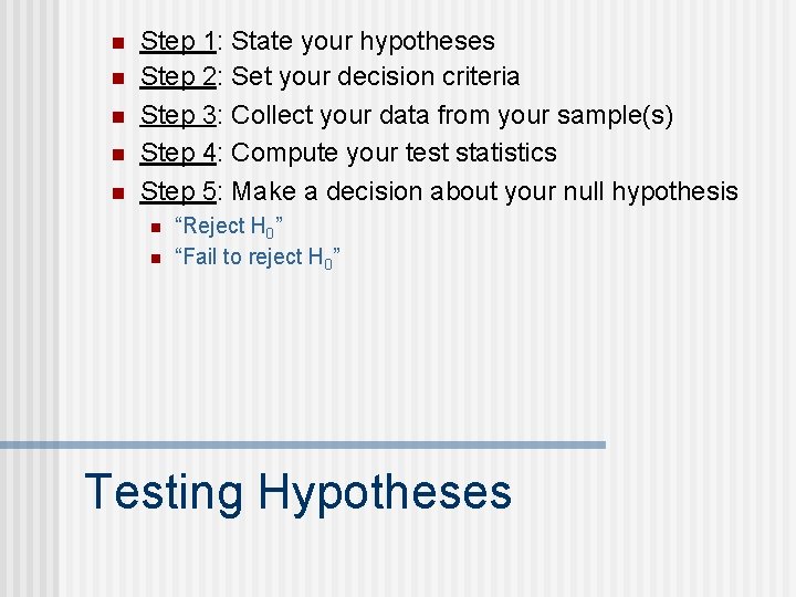
n n n Step 1: State your hypotheses Step 2: Set your decision criteria Step 3: Collect your data from your sample(s) Step 4: Compute your test statistics Step 5: Make a decision about your null hypothesis n n “Reject H 0” “Fail to reject H 0” Testing Hypotheses

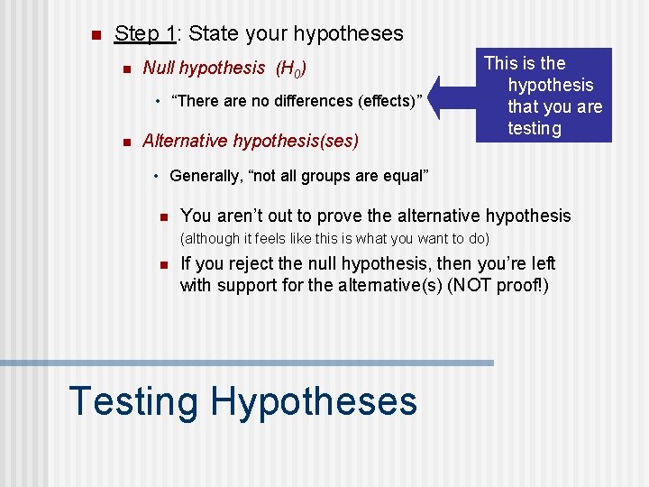
n Step 1: State your hypotheses n Null hypothesis (H 0) • “There are no differences (effects)” n Alternative hypothesis(ses) This is the hypothesis that you are testing • Generally, “not all groups are equal” n You aren’t out to prove the alternative hypothesis (although it feels like this is what you want to do) n If you reject the null hypothesis, then you’re left with support for the alternative(s) (NOT proof!) Testing Hypotheses

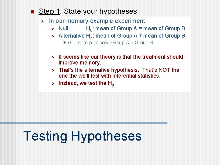
n Step 1: State your hypotheses Ø In our memory example experiment Ø Ø Null H 0: mean of Group A = mean of Group B Alternative HA: mean of Group A ≠ mean of Group B Ø (Or more precisely: Group A > Group B) Ø Ø Ø It seems like our theory is that the treatment should improve memory. That’s the alternative hypothesis. That’s NOT the one the we’ll test with inferential statistics. Instead, we test the H 0 Testing Hypotheses

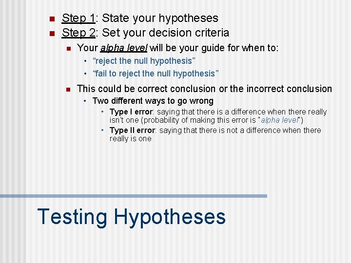
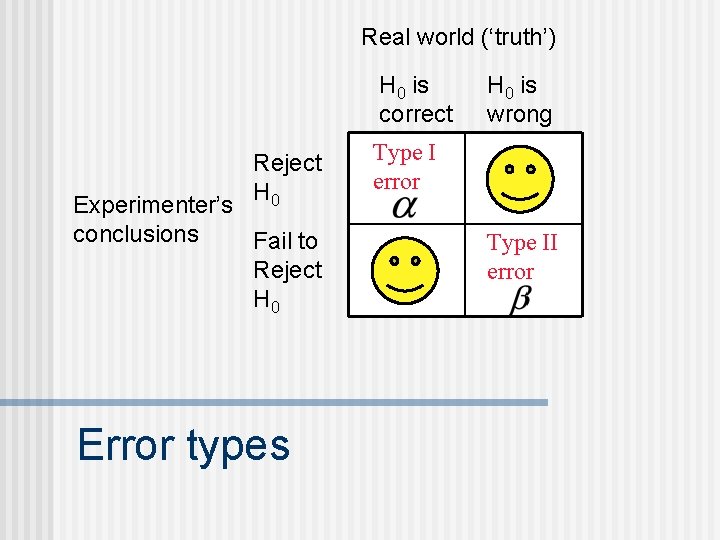
n n Step 1: State your hypotheses Step 2: Set your decision criteria n Your alpha level will be your guide for when to: • “reject the null hypothesis” • “fail to reject the null hypothesis” n This could be correct conclusion or the incorrect conclusion • Two different ways to go wrong • Type I error: saying that there is a difference when there really isn’t one (probability of making this error is “alpha level”) • Type II error: saying that there is not a difference when there really is one Testing Hypotheses

Real world (‘truth’) H 0 is correct Reject H 0 Experimenter’s conclusions Fail to Reject H 0 Error types H 0 is wrong Type I error Type II error

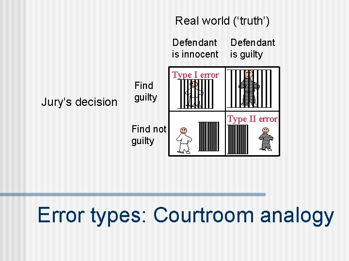
Real world (‘truth’) Defendant is innocent Defendant is guilty Type I error Jury’s decision Find guilty Find not guilty Type II error Error types: Courtroom analogy

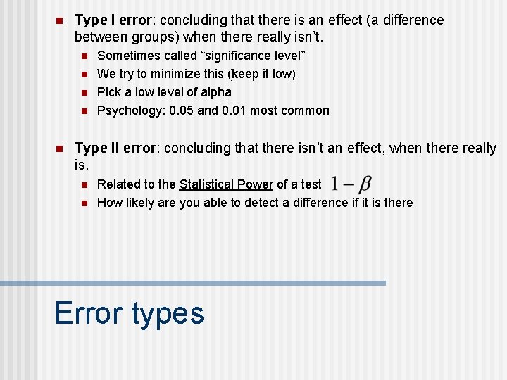
n Type I error: concluding that there is an effect (a difference between groups) when there really isn’t. n n n Sometimes called “significance level” We try to minimize this (keep it low) Pick a low level of alpha Psychology: 0. 05 and 0. 01 most common Type II error: concluding that there isn’t an effect, when there really is. n n Related to the Statistical Power of a test How likely are you able to detect a difference if it is there Error types

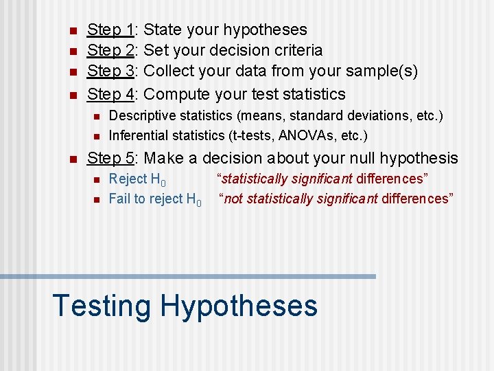
n n Step 1: State your hypotheses Step 2: Set your decision criteria Step 3: Collect your data from your sample(s) Step 4: Compute your test statistics n n n Descriptive statistics (means, standard deviations, etc. ) Inferential statistics (t-tests, ANOVAs, etc. ) Step 5: Make a decision about your null hypothesis n n Reject H 0 Fail to reject H 0 “statistically significant differences” “not statistically significant differences” Testing Hypotheses

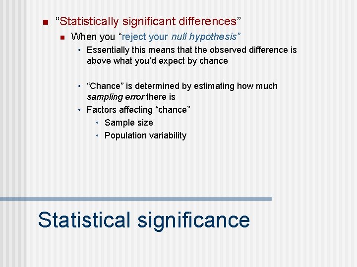
n “Statistically significant differences” n When you “reject your null hypothesis” • Essentially this means that the observed difference is above what you’d expect by chance • “Chance” is determined by estimating how much sampling error there is • Factors affecting “chance” • Sample size • Population variability Statistical significance

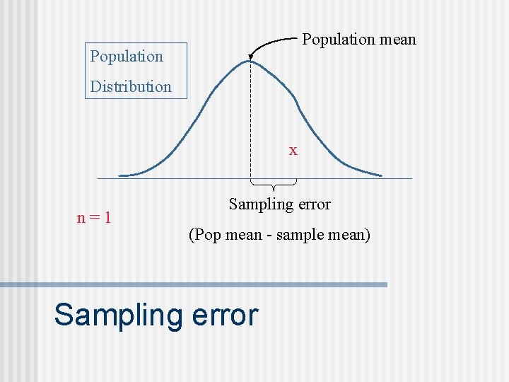
Population mean Population Distribution x n=1 Sampling error (Pop mean - sample mean) Sampling error

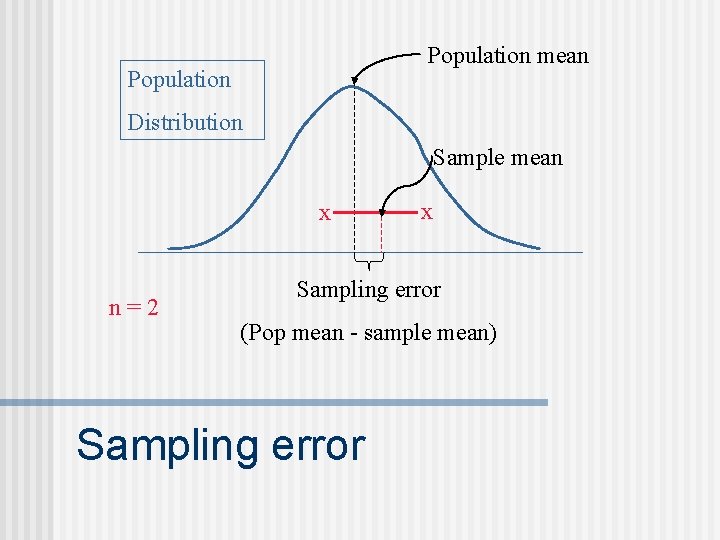
Population mean Population Distribution Sample mean x n=2 x Sampling error (Pop mean - sample mean) Sampling error

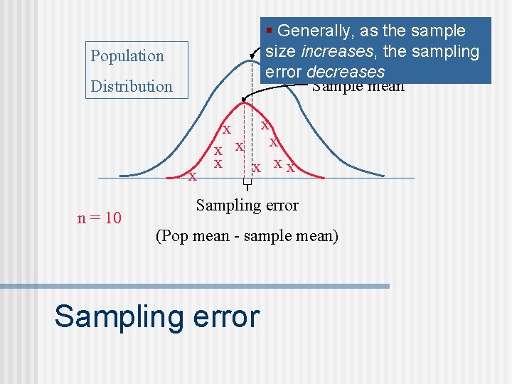
§ Generally, as mean the sample Population size increases, the sampling error decreases Sample mean Population Distribution x x n = 10 x x x xx Sampling error (Pop mean - sample mean) Sampling error

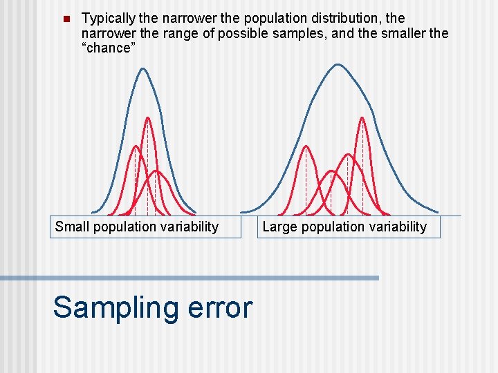
n Typically the narrower the population distribution, the narrower the range of possible samples, and the smaller the “chance” Small population variability Sampling error Large population variability

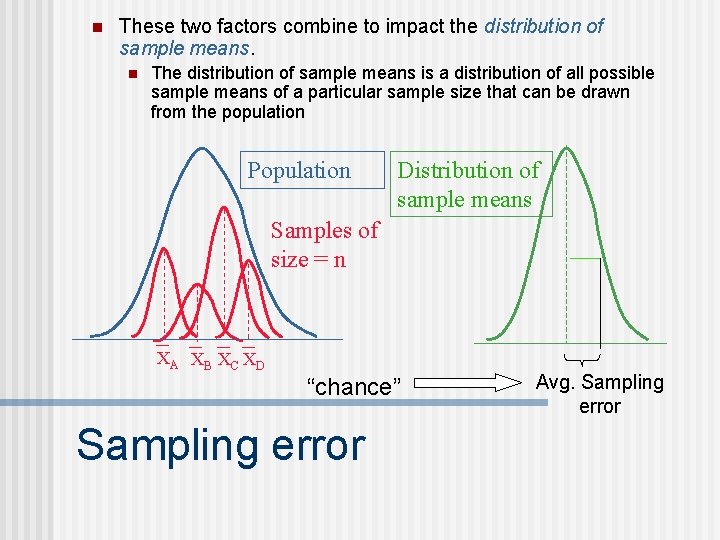
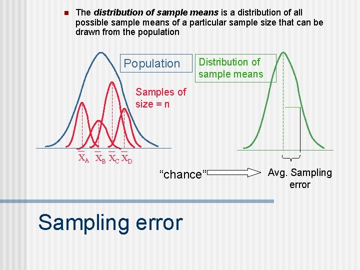
n These two factors combine to impact the distribution of sample means. n The distribution of sample means is a distribution of all possible sample means of a particular sample size that can be drawn from the population Population Distribution of sample means Samples of size = n XA XB XC XD “chance” Sampling error Avg. Sampling error

n “A statistically significant difference” means: n n n the researcher is concluding that there is a difference above and beyond chance with the probability of making a type I error at 5% (assuming an alpha level = 0. 05) Note “statistical significance” is not the same thing as theoretical significance. n n Only means that there is a statistical difference Doesn’t mean that it is an important difference Significance

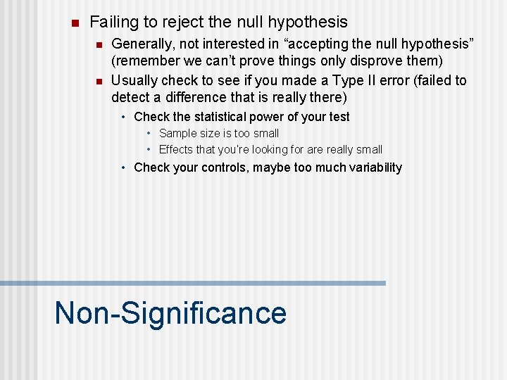
n Failing to reject the null hypothesis n n Generally, not interested in “accepting the null hypothesis” (remember we can’t prove things only disprove them) Usually check to see if you made a Type II error (failed to detect a difference that is really there) • Check the statistical power of your test • Sample size is too small • Effects that you’re looking for are really small • Check your controls, maybe too much variability Non-Significance

Ø Example Experiment: Ø Group A - gets treatment to improve memory Ø Group B - gets no treatment (control) Ø After treatment period test both groups for memory Ø Results: Ø Group A’s average memory score is 80% Ø Group B’s is 76% Ø Is the 4% difference a “real” difference (statistically significant) or is it just sampling error? Two sample distributions Experimenter’s conclusions XB XA 76% 80% From last time About populations H 0 : μ A = μ B H 0: there is no difference between Grp A and Grp B Reject H 0 Fail to Reject H 0 Real world (‘truth’) H 0 is correct H 0 is wrong Type I error Type II error

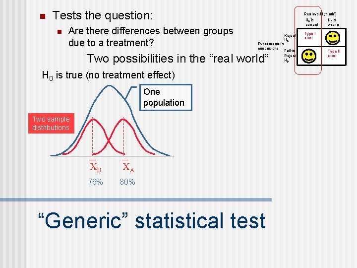
n Tests the question: n Are there differences between groups due to a treatment? Real world (‘truth’) H 0 is correct Reject H 0 Experimenter’s conclusions Fail to Reject H 0 Two possibilities in the “real world” H 0 is true (no treatment effect) One population Two sample distributions XB XA 76% 80% “Generic” statistical test H 0 is wrong Type I error Type II error

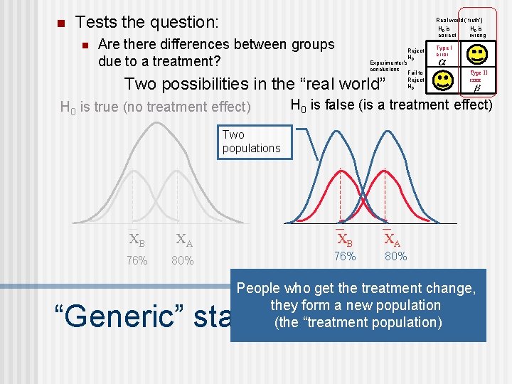
n Tests the question: n Real world (‘truth’) H 0 is correct Are there differences between groups due to a treatment? Reject H 0 Experimenter’s conclusions Fail to Reject H 0 Two possibilities in the “real world” H 0 is true (no treatment effect) H 0 is wrong Type I error Type II error H 0 is false (is a treatment effect) Two populations XB XA 76% 80% People who get the treatment change, they form a new population (the “treatment population) “Generic” statistical test

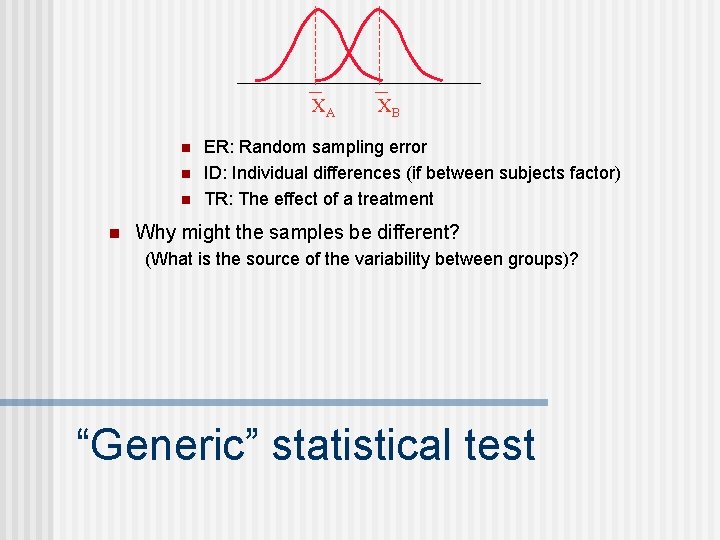
XA n n XB ER: Random sampling error ID: Individual differences (if between subjects factor) TR: The effect of a treatment Why might the samples be different? (What is the source of the variability between groups)? “Generic” statistical test

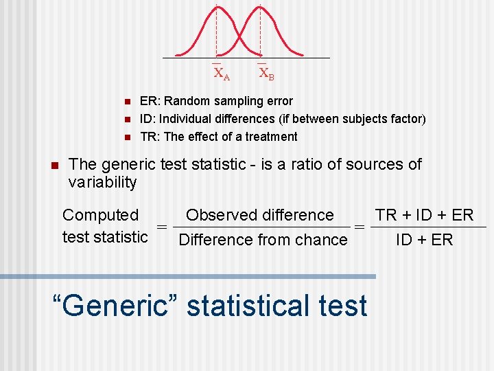
XA n n XB ER: Random sampling error ID: Individual differences (if between subjects factor) TR: The effect of a treatment The generic test statistic - is a ratio of sources of variability TR + ID + ER Observed difference Computed = = test statistic Difference from chance ID + ER “Generic” statistical test

n The distribution of sample means is a distribution of all possible sample means of a particular sample size that can be drawn from the population Population Distribution of sample means Samples of size = n XA XB XC XD “chance” Sampling error Avg. Sampling error

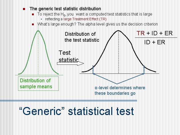
n The generic test statistic distribution n To reject the H 0, you want a computed test statistics that is large • reflecting a large Treatment Effect (TR) n What’s large enough? The alpha level gives us the decision criterion Distribution of the test statistic TR + ID + ER Test statistic Distribution of sample means α-level determines where these boundaries go “Generic” statistical test

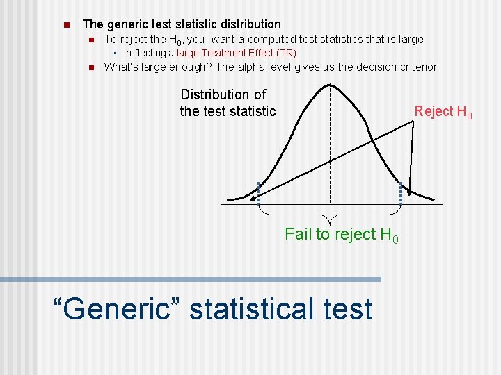
n The generic test statistic distribution n To reject the H 0, you want a computed test statistics that is large • reflecting a large Treatment Effect (TR) n What’s large enough? The alpha level gives us the decision criterion Distribution of the test statistic Reject H 0 Fail to reject H 0 “Generic” statistical test

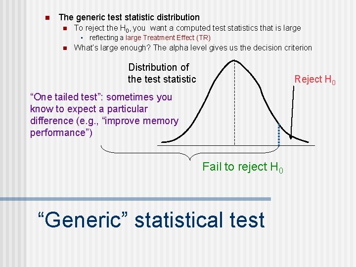
n The generic test statistic distribution n To reject the H 0, you want a computed test statistics that is large • reflecting a large Treatment Effect (TR) n What’s large enough? The alpha level gives us the decision criterion Distribution of the test statistic Reject H 0 “One tailed test”: sometimes you know to expect a particular difference (e. g. , “improve memory performance”) Fail to reject H 0 “Generic” statistical test

n Things that affect the computed test statistic n Size of the treatment effect • The bigger the effect, the bigger the computed test statistic n Difference expected by chance (sample error) • Sample size • Variability in the population “Generic” statistical test

n “A statistically significant difference” means: n n n the researcher is concluding that there is a difference above and beyond chance with the probability of making a type I error at 5% (assuming an alpha level = 0. 05) Note “statistical significance” is not the same thing as theoretical significance. n n Only means that there is a statistical difference Doesn’t mean that it is an important difference Significance

n Failing to reject the null hypothesis n n Generally, not interested in “accepting the null hypothesis” (remember we can’t prove things only disprove them) Usually check to see if you made a Type II error (failed to detect a difference that is really there) • Check the statistical power of your test • Sample size is too small • Effects that you’re looking for are really small • Check your controls, maybe too much variability Non-Significance

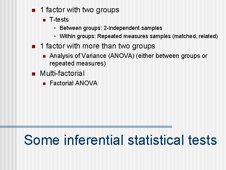
n 1 factor with two groups n T-tests • Between groups: 2 -independent samples • Within groups: Repeated measures samples (matched, related) n 1 factor with more than two groups n n Analysis of Variance (ANOVA) (either between groups or repeated measures) Multi-factorial n Factorial ANOVA Some inferential statistical tests

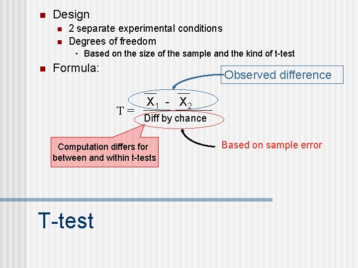
n Design n n 2 separate experimental conditions Degrees of freedom • Based on the size of the sample and the kind of t-test n Formula: Observed difference T= X 1 - X 2 Diff by chance Computation differs for between and within t-tests T-test Based on sample error

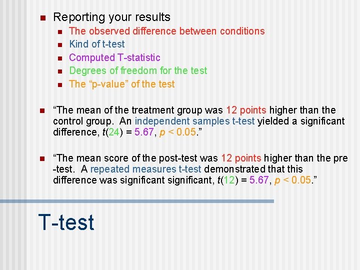
n Reporting your results n n n The observed difference between conditions Kind of t-test Computed T-statistic Degrees of freedom for the test The “p-value” of the test n “The mean of the treatment group was 12 points higher than the control group. An independent samples t-test yielded a significant difference, t(24) = 5. 67, p < 0. 05. ” n “The mean score of the post-test was 12 points higher than the pre -test. A repeated measures t-test demonstrated that this difference was significant, t(12) = 5. 67, p < 0. 05. ” T-test

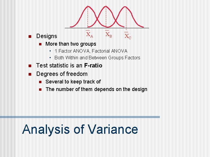
n Designs n XA XB XC More than two groups • 1 Factor ANOVA, Factorial ANOVA • Both Within and Between Groups Factors n n Test statistic is an F-ratio Degrees of freedom n n Several to keep track of The number of them depends on the design Analysis of Variance

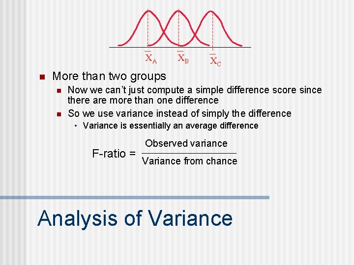
XA n XB XC More than two groups n n Now we can’t just compute a simple difference score since there are more than one difference So we use variance instead of simply the difference • Variance is essentially an average difference F-ratio = Observed variance Variance from chance Analysis of Variance

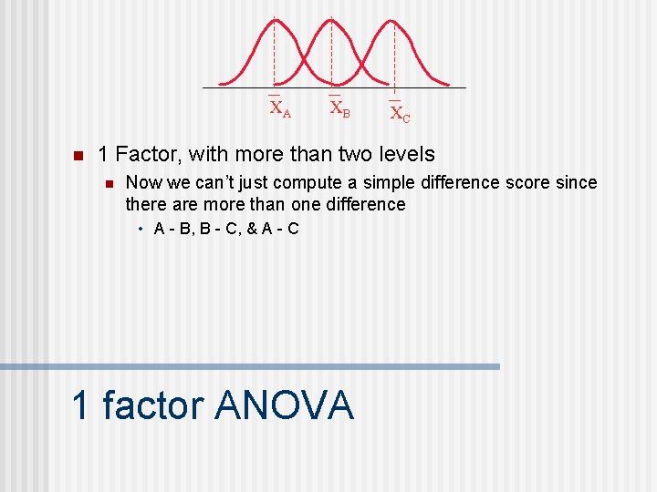
XA n XB XC 1 Factor, with more than two levels n Now we can’t just compute a simple difference score since there are more than one difference • A - B, B - C, & A - C 1 factor ANOVA

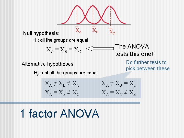
Null hypothesis: XA XB H 0: all the groups are equal XA = X B = X C Alternative hypotheses HA: not all the groups are equal XA ≠ X B ≠ X C XA = X B ≠ X C 1 factor ANOVA XC The ANOVA tests this one!! Do further tests to pick between these XA ≠ X B = X C XA = X C ≠ X B

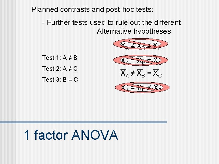
Planned contrasts and post-hoc tests: - Further tests used to rule out the different Alternative hypotheses XA ≠ X B ≠ X C Test 1: A ≠ B Test 2: A ≠ C Test 3: B = C XA = X B ≠ X C XA ≠ X B = X C XA = X C ≠ X B 1 factor ANOVA

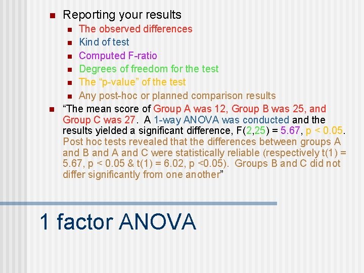
n Reporting your results The observed differences n Kind of test n Computed F-ratio n Degrees of freedom for the test n The “p-value” of the test n Any post-hoc or planned comparison results “The mean score of Group A was 12, Group B was 25, and Group C was 27. A 1 -way ANOVA was conducted and the results yielded a significant difference, F(2, 25) = 5. 67, p < 0. 05. Post hoc tests revealed that the differences between groups A and B and A and C were statistically reliable (respectively t(1) = 5. 67, p < 0. 05 & t(1) = 6. 02, p <0. 05). Groups B and C did not differ significantly from one another” n n 1 factor ANOVA

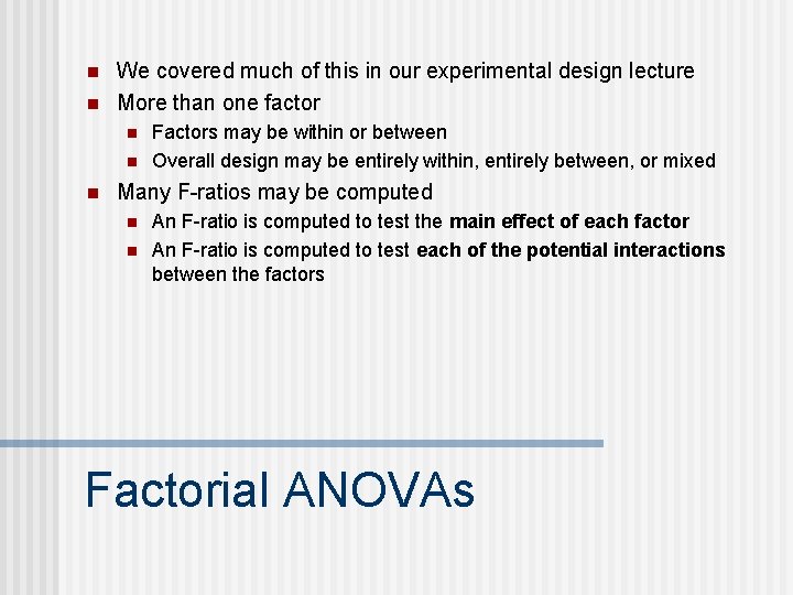
n n We covered much of this in our experimental design lecture More than one factor n n n Factors may be within or between Overall design may be entirely within, entirely between, or mixed Many F-ratios may be computed n n An F-ratio is computed to test the main effect of each factor An F-ratio is computed to test each of the potential interactions between the factors Factorial ANOVAs

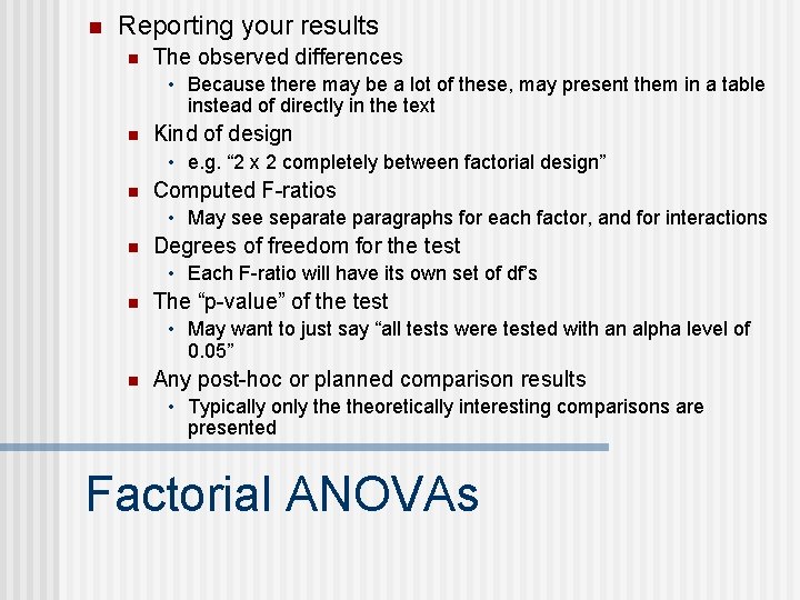
n Reporting your results n The observed differences • Because there may be a lot of these, may present them in a table instead of directly in the text n Kind of design • e. g. “ 2 x 2 completely between factorial design” n Computed F-ratios • May see separate paragraphs for each factor, and for interactions n Degrees of freedom for the test • Each F-ratio will have its own set of df’s n The “p-value” of the test • May want to just say “all tests were tested with an alpha level of 0. 05” n Any post-hoc or planned comparison results • Typically only theoretically interesting comparisons are presented Factorial ANOVAs

n Sometimes you just can’t perform a fully controlled experiment n n Because of the issue of interest Limited resources (not enough subjects, observations are too costly, etc). • Surveys • Correlational • Quasi-Experiments • Developmental designs • Small-N designs n This does NOT imply that they are bad designs n Just remember the advantages and disadvantages of each Non-Experimental designs

n What are they? n n Historically, these were the typical kind of design used until 1920’s when there was a shift to using larger sample sizes Even today, in some sub-areas, using small N designs is common place • (e. g. , psychophysics, clinical settings, animal studies, expertise, etc. ) Small N designs

n In contrast to Large N-designs (comparing aggregated performance of large groups of participants) n One or a few participants Data are typically not analyzed statistically; rather rely on visual interpretation of the data n Small N designs

= observation Steady state (baseline) Treatment introduced n n Observations begin in the absence of treatment (BASELINE) Then treatment is implemented and changes in frequency, magnitude, or intensity of behavior are recorded Small N designs

= observation Transition steady state Steady state (baseline) Treatment introduced n Treatment removed Reversibility Baseline experiments – the basic idea is to show: 1. when the IV occurs, you get the effect 2. when the IV doesn’t occur, you don’t get the effect (reversibility) Small N designs

Unstable § Stable Before introducing treatment (IV), baseline needs to be stable Measure level and trend § n Level – how frequent (how intense) is behavior? • Are all the data points high or low? n Trend – does behavior seem to increase (or decrease) • Are data points “flat” or on a slope? Small N designs

Steady state (baseline) Transition steady state n Reversibility ABA design (baseline, treatment, baseline) – The reversibility is necessary, otherwise something else may have caused the effect other than the IV (e. g. , history, maturation, etc. ) n There are other designs as well (e. g. , ABAB see figure 13. 6 in your textbook) ABA design

n Advantages n n n Focus on individual performance, not fooled by group averaging effects Focus is on big effects (small effects typically can’t be seen without using large groups) Avoid some ethical problems – e. g. , with nontreatments Allows to look at unusual (and rare) types of subjects (e. g. , case studies of amnesics, experts vs. novices) Often used to supplement large N studies, with more observations on fewer subjects Small N designs

n Disadvantages n n n Difficult to determine how generalizable the effects are Effects may be small relative to variability of situation so NEED more observation Some effects are by definition between subjects • Treatment leads to a lasting change, so you don’t get reversals Small N designs

n n Some researchers have argued that Small N designs are the best way to go. The goal of psychology is to describe behavior of an individual Looking at data collapsed over groups “looks” in the wrong place Need to look at the data at the level of the individual Small N designs