Nominal Rigidity Introduction It is also known as


 F’( • )>0, F\"( • )<0 Time is discrete. Firms produce output")
![Household’s objective function U=∑∞t=0 βt [U(Ct) +Γ(Mt/Pt) –V(Lt) ], 0 < β < 1](https://slidetodoc.com/presentation_image/b0f3317b4d3aa2545990cf7cdc5fec39/image-6.jpg "Household’s objective function U=∑∞t=0 βt [U(Ct) +Γ(Mt/Pt) –V(Lt) ], 0 < β < 1")
=Ct 1 -ϴ / 1 -ϴ ϴ >0 ϴ willingness to")
= (Mt/Pt)1 -v/1 -v, v>0 Money is a direct source of utility.")
(1 +")
ß Ct+1 -ϴ it relating current household consumption C and")


 =it/1+it U’(Ct) -----i Γ’(Mt/Pt) =(Mt/Pt)1")


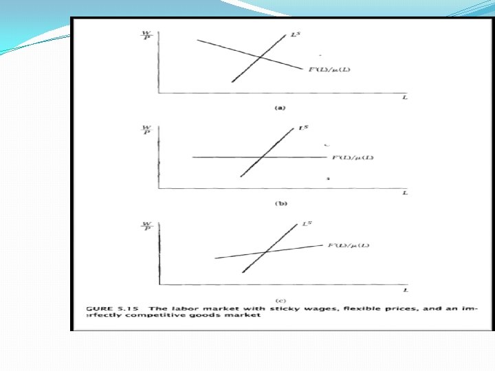
: Flexible prices, sticky wages and competitive goods market Keynes’s")


- Slides: 24
Nominal Rigidity
Introduction It is also known as price-stickiness or wage-stickiness. a situation in which the nominal price is resistant to change. Complete nominal rigidity occurs when a price is fixed in nominal terms for a relevant period of time. price of a particular good might be fixed at Rs. 10 per unit for a year. Partial nominal rigidity occurs when a price may vary in nominal terms. There are some types of barriers or limitations to the adjustment of nominal prices or wages in modern business cycle. This chapter focuses on such barriers.
There are two parts of this chapter. Part-A Ø To understand the effects of nominal rigidity and analyze the effects of various assumptions about the specifics of rigidity, such as whether it is prices or wages that are sticky and nature of inflation dynamics. Part-B Ø Microeconomics foundation of nominal Rigidity.
Part-A. Exogenous Nominal Rigidity A Baseline case: Fixed prices We take nominal rigidity as given and investigate its effects. Nominal prices are completely fixed.
Assumptions Y=f(L) F’( • )>0, F"( • )<0 Time is discrete. Firms produce output using labor as there only input. Aggregate consumption and aggregate output are equal Government and international trade are absent from the model. There is no capital.
Household’s objective function U=∑∞t=0 βt [U(Ct) +Γ(Mt/Pt) –V(Lt) ], 0 < β < 1 There is fixed number of infinitely lived households that obtain utility from consumption (U(Ct)) and from holding real money balance Γ(Mt/Pt) and disutility from working (V(Lt)). There is diminishing marginal utility of consumption and money holding and increasing marginal disutility of working.
Utility of consumption U(Ct)=Ct 1 -ϴ / 1 -ϴ ϴ >0 ϴ willingness to shift consumption between different period. When ϴ is smaller, marginal utility falls more slowly as consumption rises. C 1 -ϴ is increasing in C if ϴ < 1 but decreasing if ϴ > 1. Dividing C 1 -ϴ by 1 -ϴ ensure that marginal utility of consumption is positive regardless of the value of ϴ.
Money holding Γ(Mt/Pt)= (Mt/Pt)1 -v/1 -v, v>0 Money is a direct source of utility. Individual hold cash not because it provide utility directly but it allow to purchase some goods more easily. Two types of assets : Money: - which pays as a nominal interest rate of zero. Bonds: - which pay an interest rate of it
At+1 = Mt + (At + Wt. Lt − Pt. Ct − Mt)(1 + it). At is household wealth W is nominal wage Lt is labor Wt. Lt is labor income. Pt. Ct is Consumption expenditure. Quantity of bonds hold from t to t+1 is (At + Wt. Lt − Pt. Ct − Mt). Household take the path of P, W and i. It chose the path of C and M to maximize its lifetime utility subject to budget constraint The path of M is exogenous and path of i is determined endogenously.
Household Behavior Euler Equation Ct-ϴ=(1+rt)ß Ct+1 -ϴ it relating current household consumption C and future t household consumption C. t+1 Household reduce it consumption Ct by d. C and Increase its bond holding by changing consumption expenditure (P d. C). t r is the real interest rate t
Taking the logs of both sides and solving* for ln. Ct give us: ln. C t=ln. Ct+1 -1/ ϴln[(1+rt)ß] To get this form more use full we makes three changes: Only use output for consumption normalized the number of household to 1. In equilibrium aggregate output, Y and consumption of the household , C must be equal. Substitute Y for C. II. For small value of r, ln(1+r ) r III. Suppress the constant term, -(1/ ϴ)lnß. This can be formalized by reinterpreting r as the difference b/w the real intreset rate -ln ß. These changes give us : I. ln. Y t=ln. Yt+1 -1/ ϴrt This equation is known as new keynesian IS curve
Features of new keynesian IS curve It implies an inverse relationship between rt and yt. Demand for goods have same implication. Increase in real interest rate reduce the amount of investment.
First order condition for household optimal money holding Γ’(Mt/Pt) =it/1+it U’(Ct) -----i Γ’(Mt/Pt) =(Mt/Pt)1 -v/1 -v U’(Ct)= Ct 1 -ϴ / 1 -ϴ Ct=Yt Put these values in above equation(i) Mt/Pt=Yt ϴ/v(1+it/it)1/v The above equation describes that Money demand is increasing in output and decreasing in the nominal interest rate
The effects of shocks with fixed price Now we describe the effects of changes in the money supply and of other disturbance. We assume that prices are completely fixed both now and in future Pt = P In the absence of any type of nominal rigidity or imperfection, a change in the money supply leads to proportional change in all prices and wages, with no impact on real quantitative. Consider an increase in the money supply in period t that is fully reversed the next period, so that future output is unaffected. The increase shifts the LM curve down and does not affect the IS curve. As a result the interest rate falls and output rises. Figure *0
Price Rigidity, wage Rigidity, and Departures from perfect competition in the Goods and labor markets We will study four sets of assumptions (some combination of of nominal wage and price rigidity and characteristics of the labor and good markets) that will lead to a non-vertical AS curve. In all of these sets of assumptions, incomplete nominal adjustment is assumed not derived
Four case of assumptions Case 1 The Keynes model • Flexible prices • Sticky wages • Competitive goods market Case 3 • Sticky prices • Flexible wages • Real labor market imperfections Case 2 • Sticky prices • Flexible wages • Competitive labor market Case 4 • Flexible prices • Sticky wage • Imperfect competition
Case 1 (The Keynes Model): Flexible prices, sticky wages and competitive goods market Keynes’s General theory (1936) has two key features: First Nominal wage is completely unresponsive to current period developments. We focus on the economy in a single period. we omit time. �� = W Second Keynes did not specify explicitly, wage that prevails in the absence of nominal rigidity is above the level that equates supply and demand. Output is produced by competitive firms. Labor is the only factor of production that is variable in the short run, prices are flexible. and �� =�� (�� ) , ��′ ∙>0��′′ ∙<0 Firm hire labor up to the point where the marginal product of labor equal the real wage. F’(L)=W/P With these assumptions, increase in demand raises output through its impact on real wage. . When the money supply or some other determinant of demand rises, goods prices rises, and the real wages fall and employment rises Explain through figure *1
Case 2: Sticky prices, flexible wages and a competitive labor market Labor market is competitive and wages are completely flexible and source of incomplete nominal adjustment is entirely in the goods market. Assume that Prices are rigid. P=P Wages are flexible and labor market is competitive. Thus workers chose their labor supply to maximize utility taking the real wages as given. The first order condition for labor supply is: C-ϴ W/P=V’(L) In equilibrium, C=Y=F(L), put the value of C in above equation : W/P=[F(L)] ϴ V’(L) The right hand side of this expression is increasing in L. thus implicitly defines L as an increasing function of the real wage: L=L s(W/P), Ls’ ( • )>0 Firms meet demand at the prevailing price as long as it does not exceed the level where marginal cost equals price. With these assumptions, fluctuations in demand cause firm to change employment and output at the fixed price level. Explain by figure *2
Ratio of price to marginal cost: in response to demand fluctuations, a rise in demand leads to rise in costs, both because the wage rises and marginal product of labor declines as output rises, price stay fixed and so the ratio of price to marginal cost fall.
Case 3: Sticky prices, flexible wages and real labor market imperfections Output fluctuations appear to be associated with employment fluctuations, we can ask if movements in AD can affect unemployment when it is nominal prices that are sluggish. This case extends Case 2 by introducing real imperfections in the labor market. Assume that nominal wages are flexible but there are market imperfection in the labor market that causes the real wage to remain above the level that equates supply and demand. Also assume that firms have some “real-wage function”, (we can think that firms pay more than market clearing wages for efficiency wage reasons) �� /�� =�� (L) w′(∙) ≥ 0
Inflation is fixed at �� and the production function is �� =�� (�� ). Employment and real wage is now determined by the intersection of the effective labor demand the real-wage function. ◦In this case, there is unemployment. The unemployment is the distance between E and A. Further, fluctuations in labor demand lead to movement along the real-wage function and not the labor supply curve. If the real-wage function is flatter than the labor supply curve, unemployment rises when demand falls. Figure *3
Case 4: Flexible prices, sticky wages and imperfect competition This case extends Case 1 by introducing real imperfections in the goods market. The goods market is imperfectly competitive with imperfect competition: shown as price as a mark up over marginal cost. Assume a “markup function” �� =�� (�� )�� /��′ (�� ) Where �� is the markup and �� /��′ (�� ) is the marginal cost. The real wage , W/P is given by ��′ (�� )�� (�� ) without any restriction on �� (�� ). When �� (�� ) is precisely as countercyclical as ��′ (�� ). In this situation , real wage is not affected by changes in L. since nominal wages is unaffected by L by assumption, the price level is unaffected as well. If �� (�� is more countercyclical than ��′ (�� ) , then P must be lower when L is higher. Employment continues to be determined by effective labor demand. Implications for the labor market. The real wage equals ��′ (�� )/�� (�� ) which can be decreasing in L ( panal a), constant (panal b) and increasing (panal c)
A permanent output-inflation Tradeoff To build a model we need to relax the assumption that nominal prices or wages never change. one natural way to do this is to suppose that the level at which current prices or wages are fixed is determined by what happened the previous period. Model of supply: This is the model with fixed wages, flexible prices and a competitive goods market. W is to the previous period’s price level. Suppose that wages are adjusted to make up for the previous period inflation: W t=APt-1 A>0 our first model of supply, employment is determined by F’(L)=W t/Pt . The above equation for Wt is : F’(L t ) = APt-1 / Pt = A/1+ ∏t where ∏t is the inflation rate. The above equation implies a stable, upward slopping relationship between employment (and hence output) and inflation. There is a permanent output-inflation tradeoff. By accepting higher inflation, policymakers can permanently raise output, higher output is associated with lower unemployment, it is also implies a permanent unemployment-inflation tradeoff.