Noise Adjusted Principal Component Transform NAPC Data are

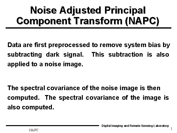
Noise Adjusted Principal Component Transform (NAPC) Data are first preprocessed to remove system bias by subtracting dark signal. This subtraction is also applied to a noise image. The spectral covariance of the noise image is then computed. The spectral covariance of the image is also computed. Digital Imaging and Remote Sensing Laboratory NAPC 1

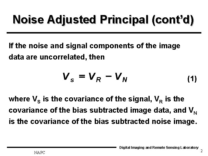
Noise Adjusted Principal (cont’d) If the noise and signal components of the image data are uncorrelated, then Vs = VR - VN (1) where VS is the covariance of the signal, VR is the covariance of the bias subtracted image data, and VN is the covariance of the bias subtracted noise image. Digital Imaging and Remote Sensing Laboratory NAPC 2

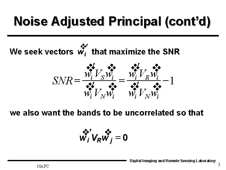
Noise Adjusted Principal (cont’d) v We seek vectors w i that maximize the SNR ¢ v v wi VS wi wi VR wi = -1 SNR = ¢ ¢ v v w. V w i N i we also want the bands to be uncorrelated so that v v = w i VRw j 0 Digital Imaging and Remote Sensing Laboratory NAPC 3

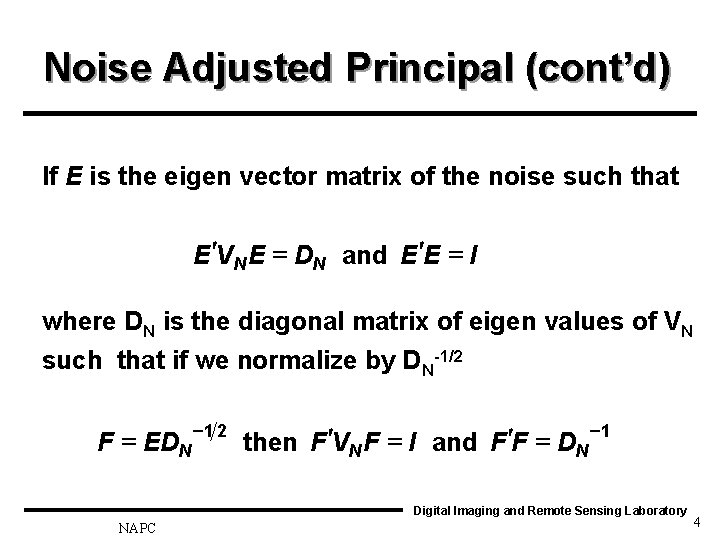
Noise Adjusted Principal (cont’d) If E is the eigen vector matrix of the noise such that E VN E = DN and E E = I where DN is the diagonal matrix of eigen values of VN such that if we normalize by DN-1/2 F = EDN -1 2 -1 then F VN F = I and F F = DN Digital Imaging and Remote Sensing Laboratory NAPC 4

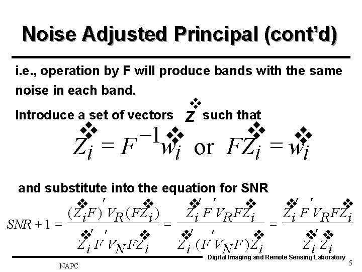
Noise Adjusted Principal (cont’d) i. e. , operation by F will produce bands with the same noise in each band. v Introduce a set of vectors Z such that v v v 1 v Zi = F wi or FZi = wi and substitute into the equation for SNR v ¢ v v¢ ¢ v ( Z i F ) VR ( FZ i ) Z i F VR FZ i = = SNR + 1 = v¢ ¢ v v¢ v Z i F VN FZ i ( F VN F ) Z i Zi Zi Digital Imaging and Remote Sensing Laboratory NAPC 5

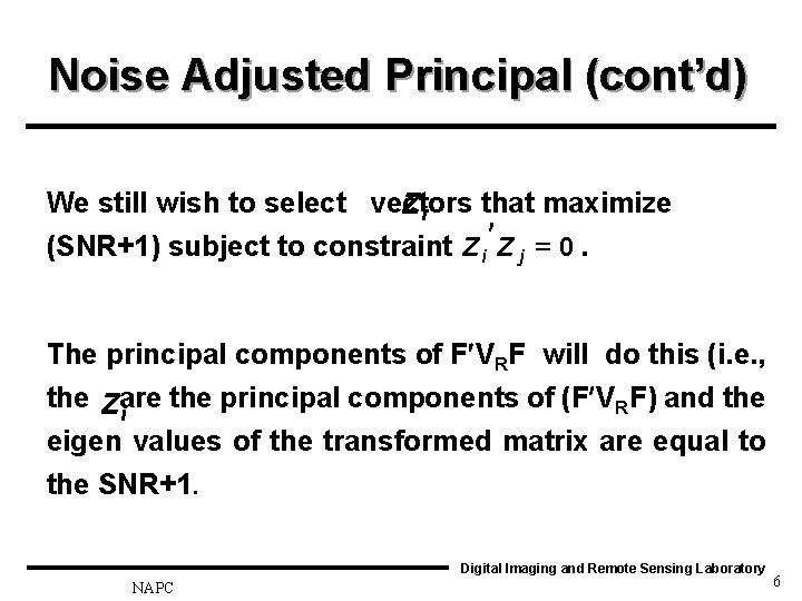
Noise Adjusted Principal (cont’d) We still wish to select vectors that maximize Zi (SNR+1) subject to constraint Z i Z j = 0. The principal components of F VRF will do this (i. e. , the Zare the principal components of (F VRF) and the i eigen values of the transformed matrix are equal to the SNR+1. Digital Imaging and Remote Sensing Laboratory NAPC 6

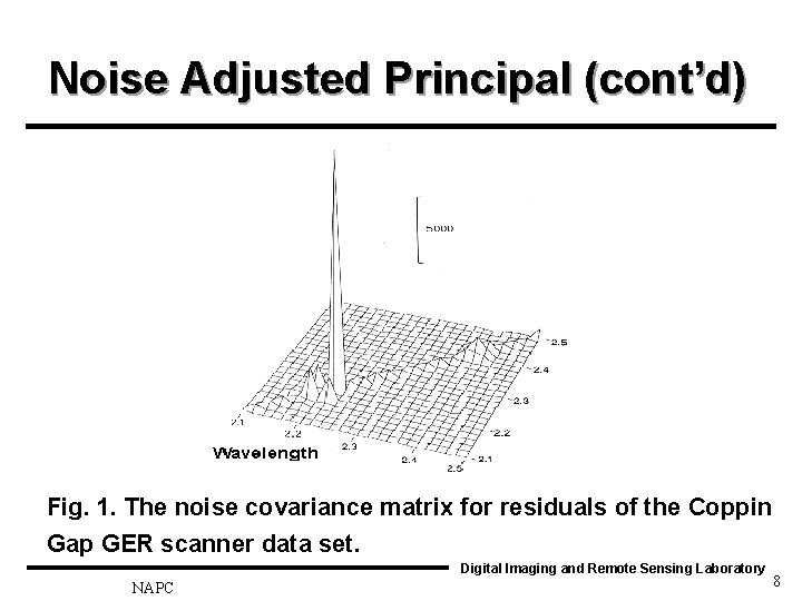
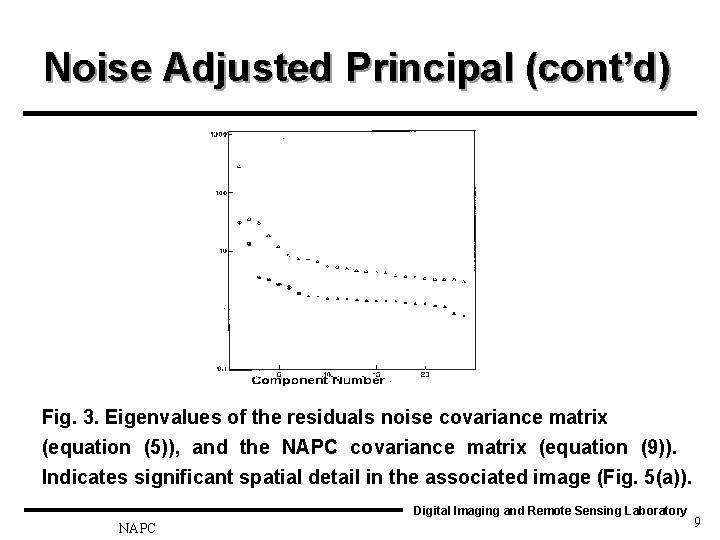
Noise Adjusted Principal (cont’d) The utility of this approach is shown in Figure 1 where noise is shown to be correlated between bands which simple noise scaling will not account for (N. B. residuals are pixel values after initial calibration). Figure 3 shows how NAPC eigen values approach 1 (SNR+1) after several NAPC bands as expected and images show spatial detail in first N images with little spatial noise. Digital Imaging and Remote Sensing Laboratory NAPC 7

Noise Adjusted Principal (cont’d) Fig. 1. The noise covariance matrix for residuals of the Coppin Gap GER scanner data set. Digital Imaging and Remote Sensing Laboratory NAPC 8

Noise Adjusted Principal (cont’d) Fig. 3. Eigenvalues of the residuals noise covariance matrix (equation (5)), and the NAPC covariance matrix (equation (9)). Indicates significant spatial detail in the associated image (Fig. 5(a)). Digital Imaging and Remote Sensing Laboratory NAPC 9

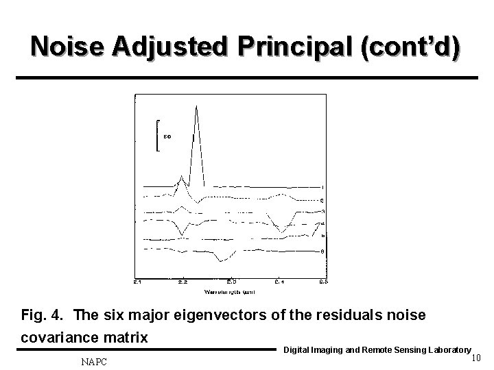
Noise Adjusted Principal (cont’d) Fig. 4. The six major eigenvectors of the residuals noise covariance matrix Digital Imaging and Remote Sensing Laboratory NAPC 10

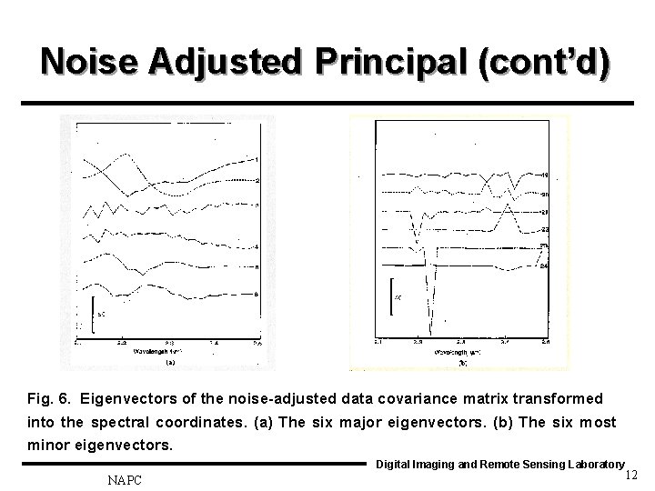
Noise Adjusted Principal (cont’d) Note in some NAPC bands (3 and 4 in this analysis) show edge effects due to spectral misregistration (attributed to timing in adjacent bands) this is not removed by this process since the processing is spectral, not spatial. Note how in Figure 6 it shows up as a saw tooth in the eigen value weights in the v original spectral space (FZ i ). Digital Imaging and Remote Sensing Laboratory NAPC 11

Noise Adjusted Principal (cont’d) Fig. 6. Eigenvectors of the noise-adjusted data covariance matrix transformed into the spectral coordinates. (a) The six major eigenvectors. (b) The six most minor eigenvectors. Digital Imaging and Remote Sensing Laboratory NAPC 12

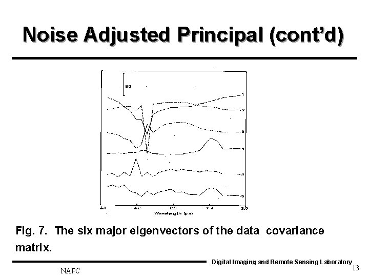
Noise Adjusted Principal (cont’d) Fig. 7. The six major eigenvectors of the data covariance matrix. Digital Imaging and Remote Sensing Laboratory NAPC 13

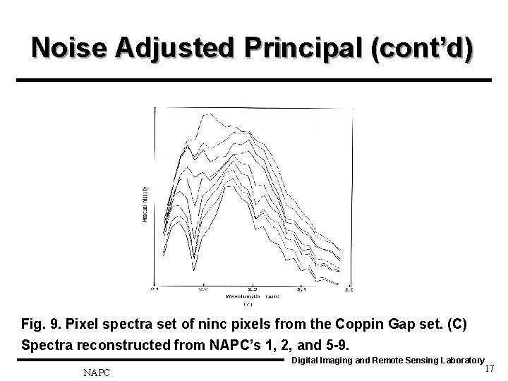
Noise Adjusted Principal (cont’d) Note, similarities between the early noise eigen vector weights Figure 4 and last eigen vector weights of the NAPC (Figure 6) and the first PC weights of the unprocessed image data (Figure 7). Also note, the saw tooth in bands 3 and 4 of NAPC transform. Spectral smoothing of back transform by eliminating is shown in Figure 9. Digital Imaging and Remote Sensing Laboratory NAPC 14

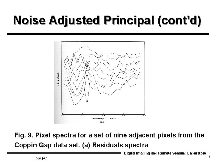
Noise Adjusted Principal (cont’d) Fig. 9. Pixel spectra for a set of nine adjacent pixels from the Coppin Gap data set. (a) Residuals spectra Digital Imaging and Remote Sensing Laboratory NAPC 15

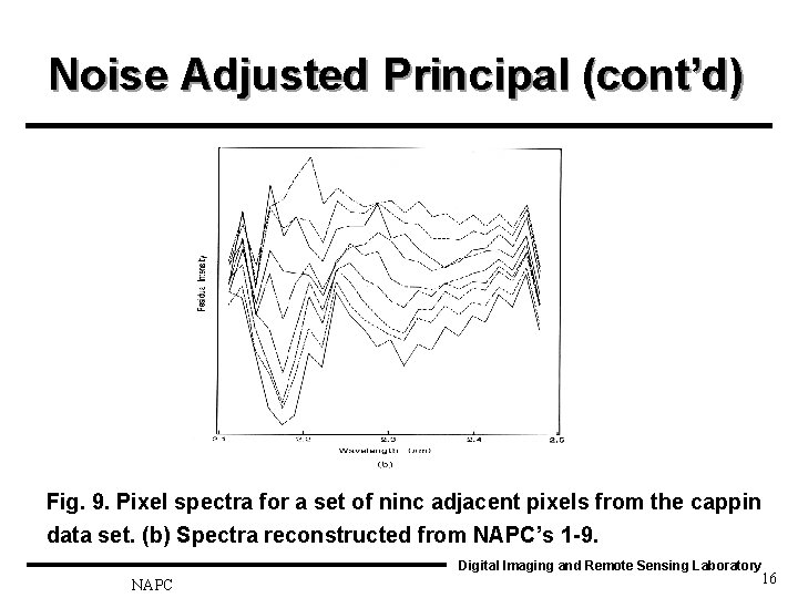
Noise Adjusted Principal (cont’d) Fig. 9. Pixel spectra for a set of ninc adjacent pixels from the cappin data set. (b) Spectra reconstructed from NAPC’s 1 -9. Digital Imaging and Remote Sensing Laboratory NAPC 16

Noise Adjusted Principal (cont’d) Fig. 9. Pixel spectra set of ninc pixels from the Coppin Gap set. (C) Spectra reconstructed from NAPC’s 1, 2, and 5 -9. Digital Imaging and Remote Sensing Laboratory NAPC 17

Noise Adjusted Principal (cont’d) Note figure 9 b has reduced random noise but still has fixed pattern noise associated with NAPC components 3 and 4 (i. e. , misregistration noise). This is eliminated in Figure 9 c. Note the importance of looking at weights on original bands where they have physical meaning!! Std. PC problems. Digital Imaging and Remote Sensing Laboratory NAPC 18