No quiz today Randomized Algorithms 2 1 BLOOM

No quiz today! Randomized Algorithms - 2 1

BLOOM FILTERS - RECAP 2

Bloom filters • Interface to a Bloom filter – Bloom. Filter(int max. Size, double p); – void bf. add(String s); // insert s – bool bd. contains(String s); • // If s was added return true; • // else with probability at least 1 -p return false; • // else with probability at most p return true; – I. e. , a noisy “set” where you can test membership (and that’s it) 3

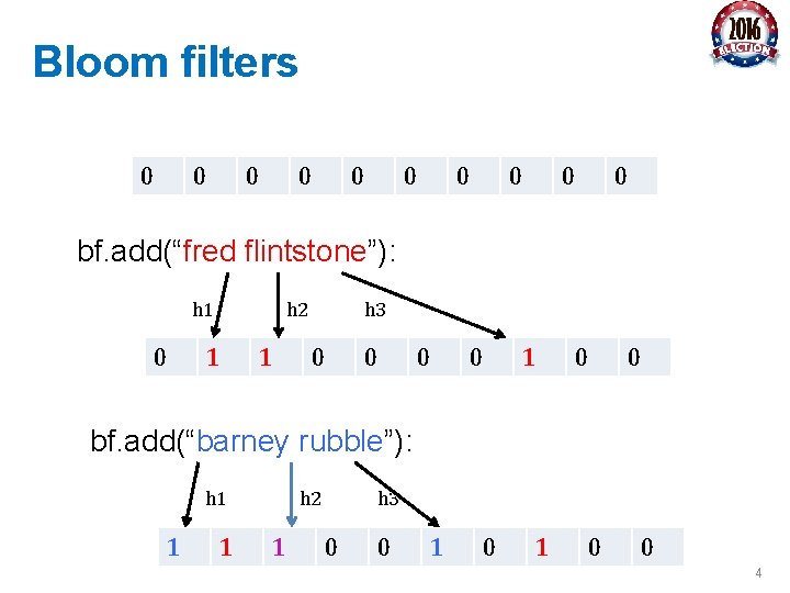
Bloom filters 0 0 0 0 0 bf. add(“fred flintstone”): h 1 0 h 2 1 1 h 3 0 0 1 0 0 bf. add(“barney rubble”): h 1 1 1 h 2 1 h 3 0 0 1 0 0 4

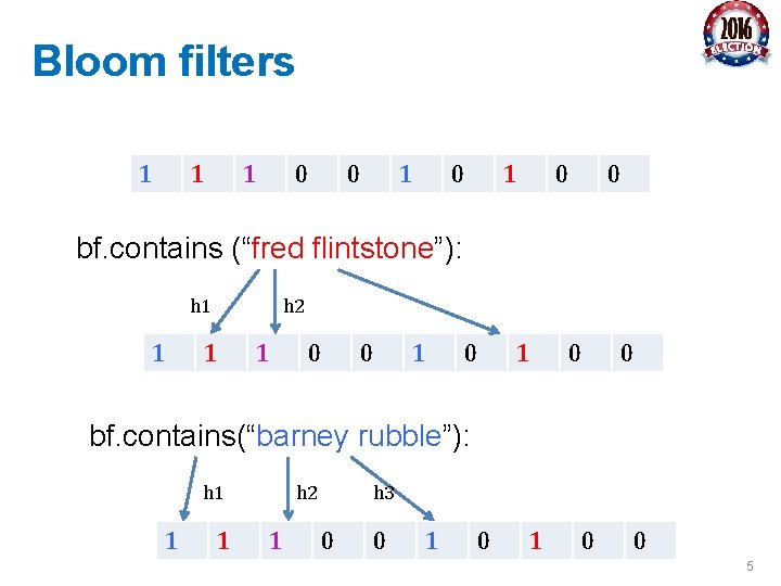
Bloom filters 1 1 1 0 0 bf. contains (“fred flintstone”): h 1 1 h 2 1 1 0 0 bf. contains(“barney rubble”): h 1 1 1 h 2 1 h 3 0 0 1 0 0 5

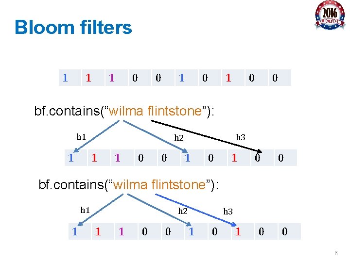
Bloom filters 1 1 1 0 0 bf. contains(“wilma flintstone”): h 1 1 h 3 h 2 1 1 0 0 bf. contains(“wilma flintstone”): h 1 1 h 2 1 1 0 0 h 3 1 0 0 6

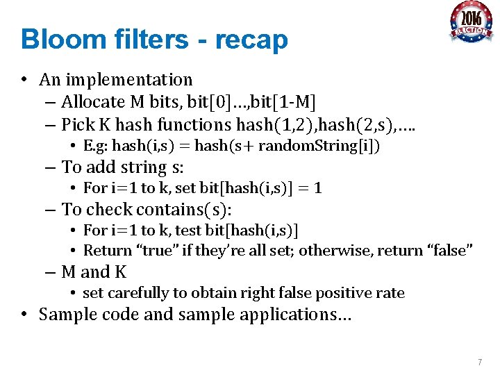
Bloom filters - recap • An implementation – Allocate M bits, bit[0]…, bit[1 -M] – Pick K hash functions hash(1, 2), hash(2, s), …. • E. g: hash(i, s) = hash(s+ random. String[i]) – To add string s: • For i=1 to k, set bit[hash(i, s)] = 1 – To check contains(s): • For i=1 to k, test bit[hash(i, s)] • Return “true” if they’re all set; otherwise, return “false” – M and K • set carefully to obtain right false positive rate • Sample code and sample applications… 7

THE COUNT-MIN SKETCH: RECAP 8

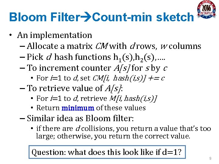
Bloom Filter Count-min sketch • An implementation – Allocate a matrix CM with d rows, w columns – Pick d hash functions h 1(s), h 2(s), …. – To increment counter A[s] for s by c • For i=1 to d, set CM[i, hash(i, s)] += c – To retrieve value of A[s]: • For i=1 to d, retrieve M[i, hash(i, s)] • Return minimum of these values – Similar idea as Bloom filter: • if there are d collisions, you return a value that’s too large; otherwise, you return the correct value. Question: what does this look like if d=1? 9

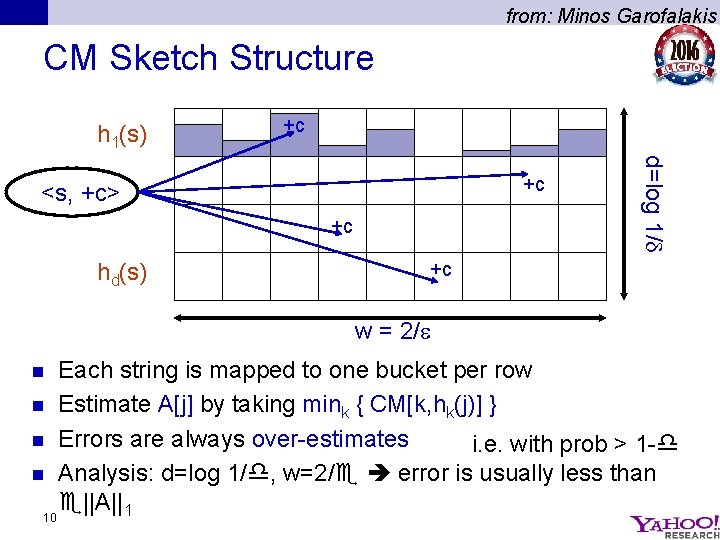
from: Minos Garofalakis CM Sketch Structure h 1(s) +c +c hd(s) d=log 1/ +c <s, +c> +c w = 2/ Each string is mapped to one bucket per row n Estimate A[j] by taking mink { CM[k, hk(j)] } n Errors are always over-estimates i. e. with prob > 1 - n Analysis: d=log 1/ , w=2/ error is usually less than ||A||1 10 n

from: Minos Garofalakis CM Sketch Guarantees [Cormode, Muthukrishnan’ 04] CM sketch guarantees approximation error on point queries less than ||A||1 in space O(1/ log 1/ ) n CM sketches are also accurate for skewed values---i. e. , only a few entries s with large A[s] – “Finding heavy hitters” n Application: – finding counts for words x, y that frequently co-occur compute “semantic orientation” of words – some others later on n A disadvantage: – CM is harder to tune than Bloom filters n 11

LOCALITY SENSITIVE HASHING (LSH) 12

13

Wait, did he say locality sensitive hash browns? 14

LSH: key ideas • Goal: – map feature vector x to bit vector bx – ensure that bx preserves “similarity” 15

Random Projections 16

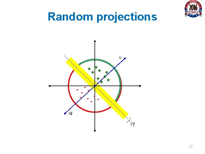
Random projections u + ++ + - -- - - -u 2γ 17

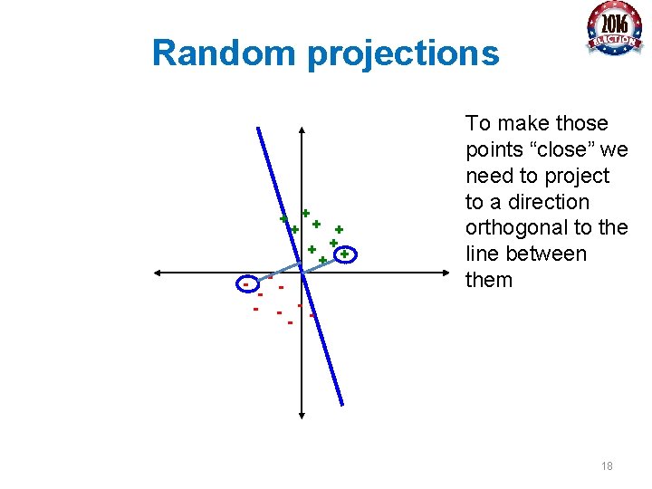
Random projections + ++ + To make those points “close” we need to project to a direction orthogonal to the line between them 18 - -- -

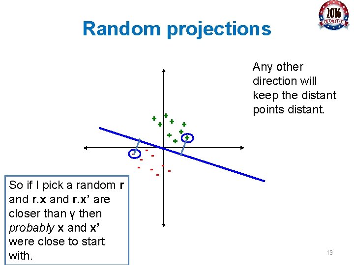
Random projections + ++ + - -- - So if I pick a random r and r. x’ are -u closer than γ then probably x and x’ were close to start with. Any other direction will keep the distant points distant. 19

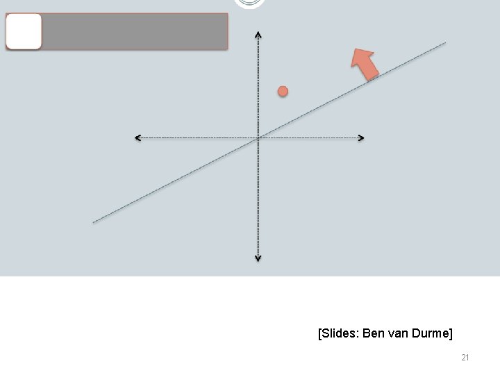
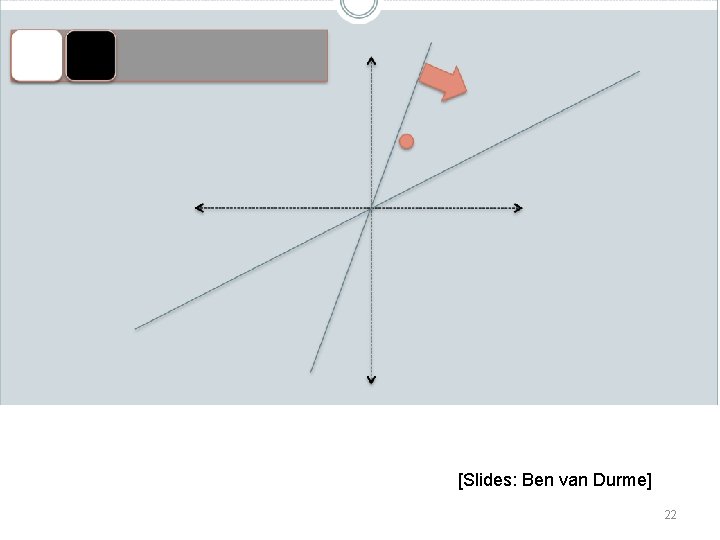
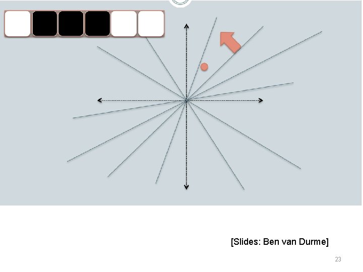
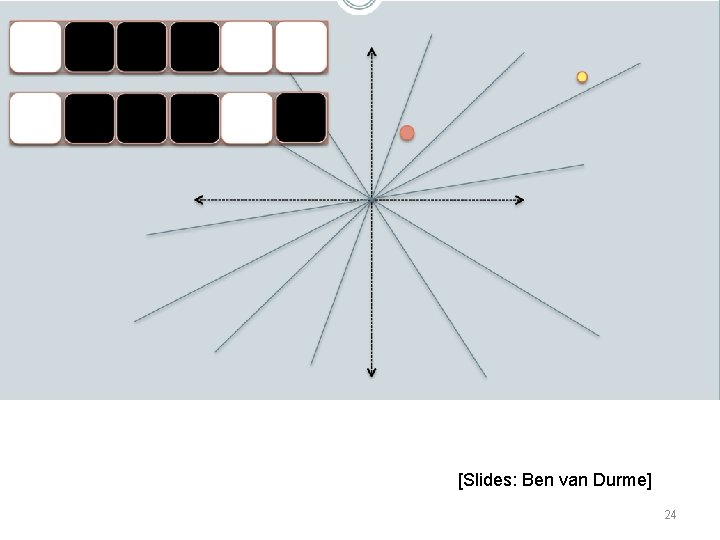
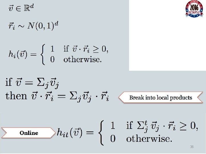
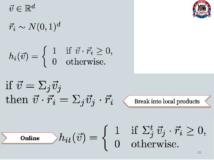
LSH: key ideas • Goal: – map feature vector x to bit vector bx – ensure that bx preserves “similarity” • Basic idea: use random projections of x – Repeat many times: • Pick a random hyperplane r by picking random weights for each feature (say from a Gaussian) • Compute the inner product of r with x • Record if x is “close to” r (r. x>=0) – the next bit in bx • Theory says that is x’ and x have small cosine distance then bx and bx’ will have small Hamming distance 20

[Slides: Ben van Durme] 21

[Slides: Ben van Durme] 22

[Slides: Ben van Durme] 23

[Slides: Ben van Durme] 24

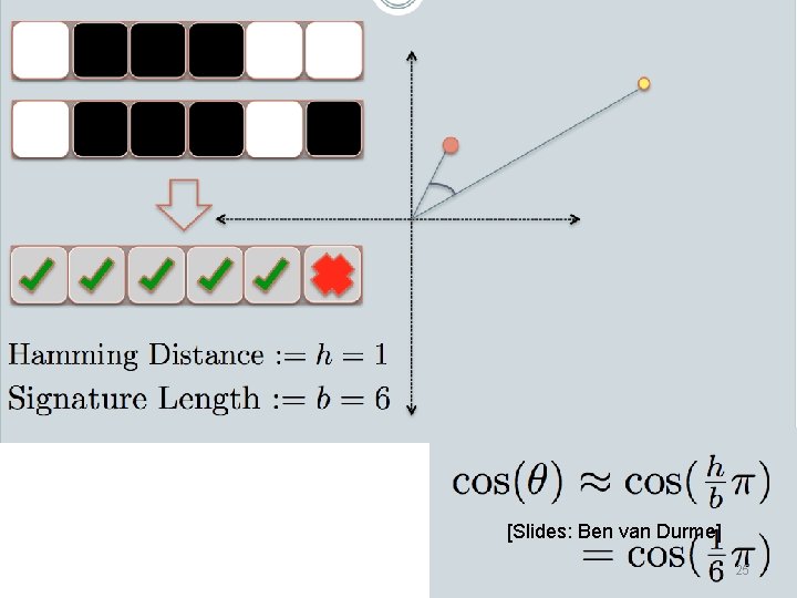
[Slides: Ben van Durme] 25

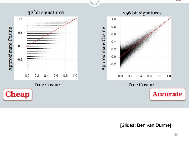
[Slides: Ben van Durme] 26

LSH applications • Compact storage of data – and we can still compute similarities • LSH also gives very fast approximations: – approx nearest neighbor method • just look at other items with bx’=bx • also very fast nearest-neighbor methods for Hamming distance – very fast clustering • cluster = all things with same bx vector 27

28

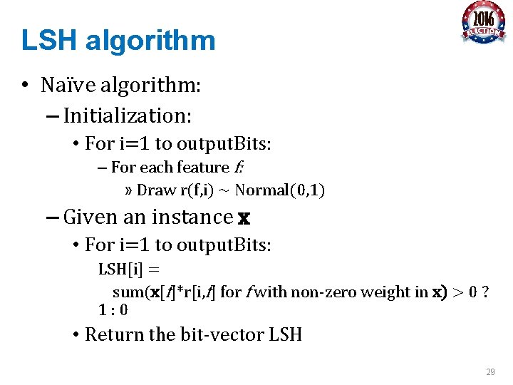
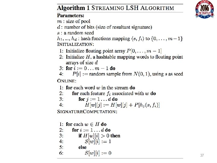
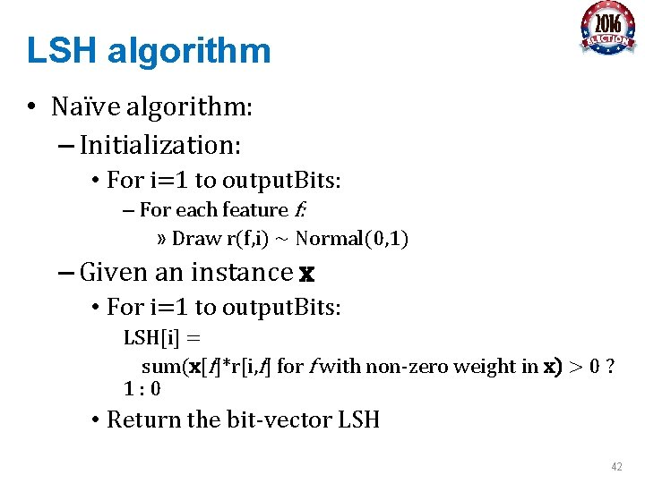
LSH algorithm • Naïve algorithm: – Initialization: • For i=1 to output. Bits: – For each feature f: » Draw r(f, i) ~ Normal(0, 1) – Given an instance x • For i=1 to output. Bits: LSH[i] = sum(x[f]*r[i, f] for f with non-zero weight in x) > 0 ? 1: 0 • Return the bit-vector LSH 29

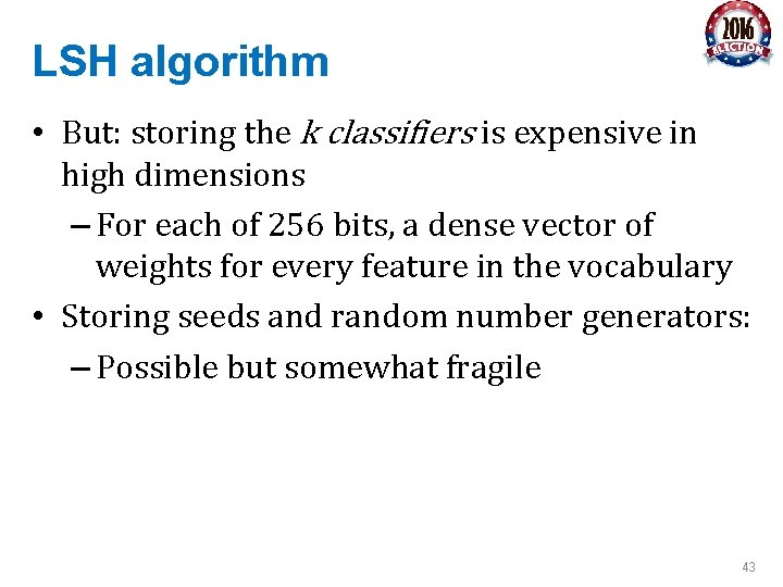
LSH algorithm • But: storing the k classifiers is expensive in high dimensions – For each of 256 bits, a dense vector of weights for every feature in the vocabulary • Storing seeds and random number generators: – Possible but somewhat fragile 30

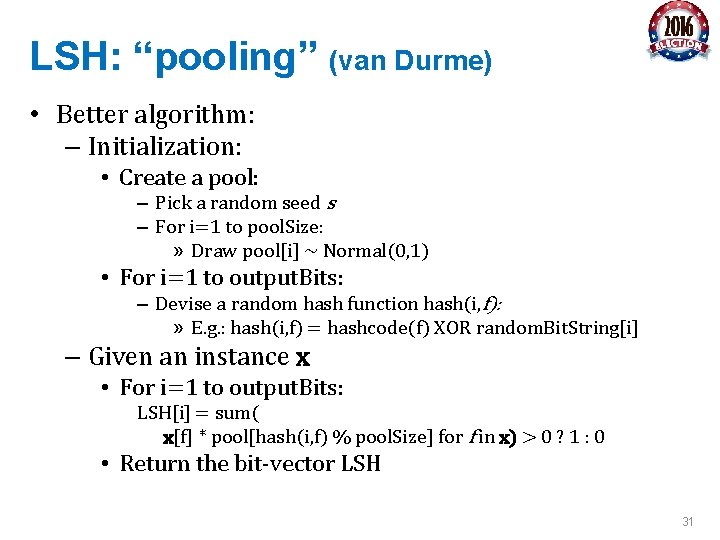
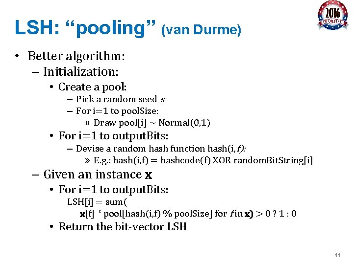
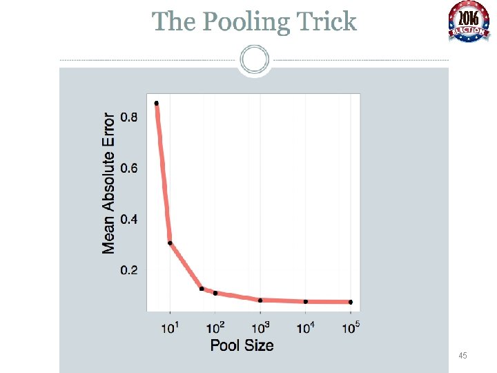
LSH: “pooling” (van Durme) • Better algorithm: – Initialization: • Create a pool: – Pick a random seed s – For i=1 to pool. Size: » Draw pool[i] ~ Normal(0, 1) • For i=1 to output. Bits: – Devise a random hash function hash(i, f): » E. g. : hash(i, f) = hashcode(f) XOR random. Bit. String[i] – Given an instance x • For i=1 to output. Bits: LSH[i] = sum( x[f] * pool[hash(i, f) % pool. Size] for f in x) > 0 ? 1 : 0 • Return the bit-vector LSH 31

32

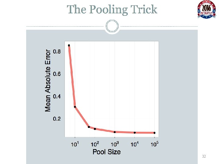
LSH: key ideas: pooling • Advantages: – with pooling, this is a compact re-encoding of the data • you don’t need to store the r’s, just the pool 33

Locality Sensitive Hashing (LSH) in an On-line Setting 34

LSH: key ideas: online computation • Common task: distributional clustering – for a word w, x(w) is sparse vector of words that co-occur with w – cluster the w’s 35

36

37

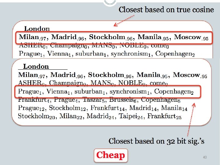
Experiment • Corpus: 700 M+ tokens, 1. 1 M distinct bigrams • For each, build a feature vector of words that co-occur near it, using on-line LSH • Check results with 50, 000 actual vectors 38

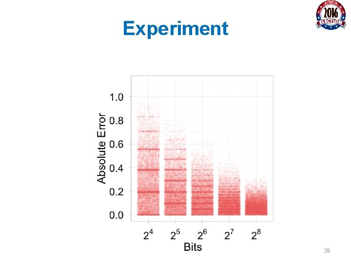
Experiment 39

40

Locality Sensitive Hashing (LSH) and Pooling Random Values 41

LSH algorithm • Naïve algorithm: – Initialization: • For i=1 to output. Bits: – For each feature f: » Draw r(f, i) ~ Normal(0, 1) – Given an instance x • For i=1 to output. Bits: LSH[i] = sum(x[f]*r[i, f] for f with non-zero weight in x) > 0 ? 1: 0 • Return the bit-vector LSH 42

LSH algorithm • But: storing the k classifiers is expensive in high dimensions – For each of 256 bits, a dense vector of weights for every feature in the vocabulary • Storing seeds and random number generators: – Possible but somewhat fragile 43

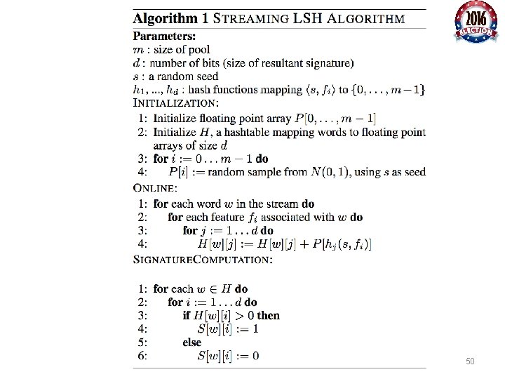
LSH: “pooling” (van Durme) • Better algorithm: – Initialization: • Create a pool: – Pick a random seed s – For i=1 to pool. Size: » Draw pool[i] ~ Normal(0, 1) • For i=1 to output. Bits: – Devise a random hash function hash(i, f): » E. g. : hash(i, f) = hashcode(f) XOR random. Bit. String[i] – Given an instance x • For i=1 to output. Bits: LSH[i] = sum( x[f] * pool[hash(i, f) % pool. Size] for f in x) > 0 ? 1 : 0 • Return the bit-vector LSH 44

45

LSH: key ideas: pooling • Advantages: – with pooling, this is a compact re-encoding of the data • you don’t need to store the r’s, just the pool 46

Locality Sensitive Hashing (LSH) in an On-line Setting 47

LSH: key ideas: online computation • Common task: distributional clustering – for a word w, x(w) is sparse vector of words that co-occur with w – cluster the w’s 48

49

50

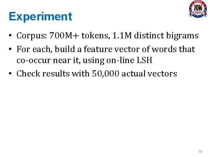
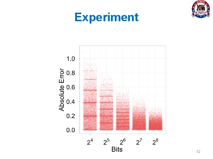
Experiment • Corpus: 700 M+ tokens, 1. 1 M distinct bigrams • For each, build a feature vector of words that co-occur near it, using on-line LSH • Check results with 50, 000 actual vectors 51

Experiment 52

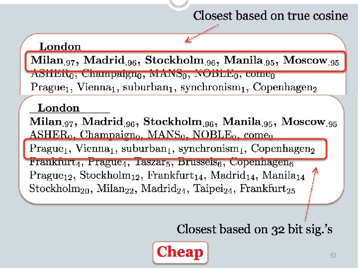
53

Points to review • APIs for: – Bloom filters, CM sketch, LSH • Key applications of: – Very compact noisy sets – Efficient counters accurate for large counts – Fast approximate cosine distance • Key ideas: – Uses of hashing that allow collisions – Random projection – Multiple hashes to control Pr(collision) – Pooling to compress a lot of random draws 54