NMR Relaxation Measurements How to measure relaxation rates

NMR: Relaxation Measurements

How to measure relaxation rates? T 1: Longitudinal or spin-lattice relaxation. Mz is restored, the system goes back to equilibrium. T 2: Transverse or spin-spin relaxation. Transverse magnetization Mx, y vanishes, the observable signal disappears. For measurements pulsed methods should be used

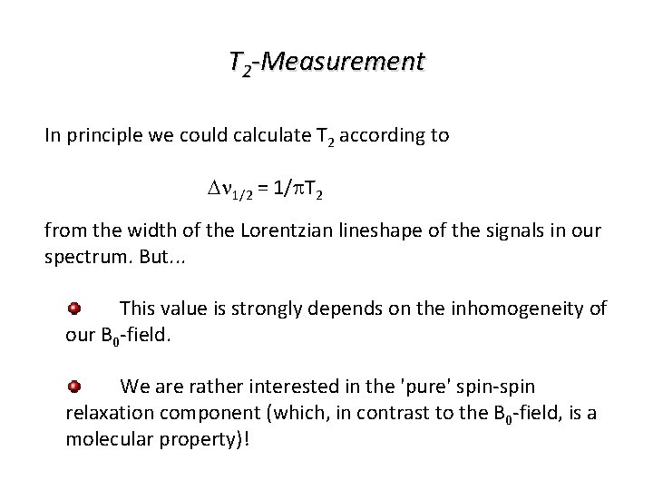
T 2 -Measurement In principle we could calculate T 2 according to Dn 1/2 = 1/p. T 2 from the width of the Lorentzian lineshape of the signals in our spectrum. But. . . This value is strongly depends on the inhomogeneity of our B 0 -field. We are rather interested in the 'pure' spin-spin relaxation component (which, in contrast to the B 0 -field, is a molecular property)!

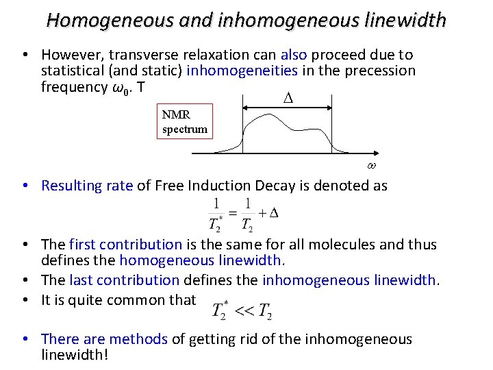
Homogeneous and inhomogeneous linewidth • However, transverse relaxation can also proceed due to statistical (and static) inhomogeneities in the precession frequency ω0. T D NMR spectrum w • Resulting rate of Free Induction Decay is denoted as • The first contribution is the same for all molecules and thus defines the homogeneous linewidth. • The last contribution defines the inhomogeneous linewidth. • It is quite common that • There are methods of getting rid of the inhomogeneous linewidth!

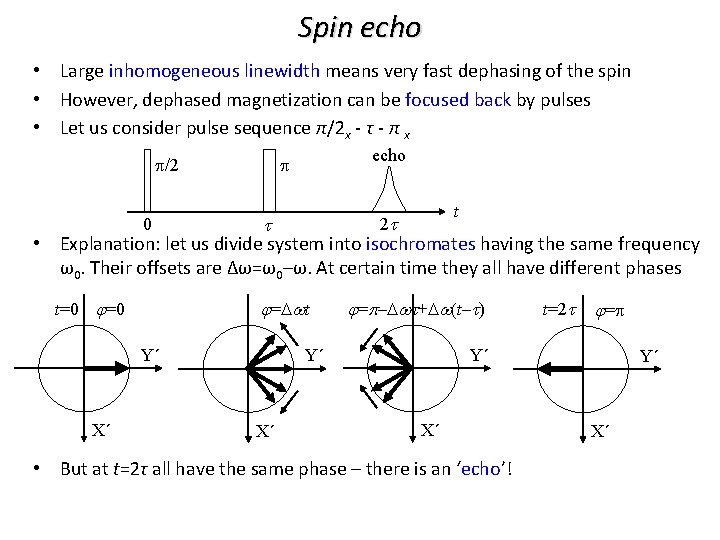
Spin echo • Large inhomogeneous linewidth means very fast dephasing of the spin • However, dephased magnetization can be focused back by pulses • Let us consider pulse sequence π/2 x - τ - π x • echo p p/2 t 2 t t Explanation: let us divide system into isochromates having the same frequency ω0. Their offsets are Δω=ω0–ω. At certain time they all have different phases 0 t=0 j=Dwt Y´ X´ j=p–Dwt+Dw(t–t) j=p Y´ Y´ X´ t=2 t X´ • But at t=2τ all have the same phase – there is an ‘echo’! Y´ X´

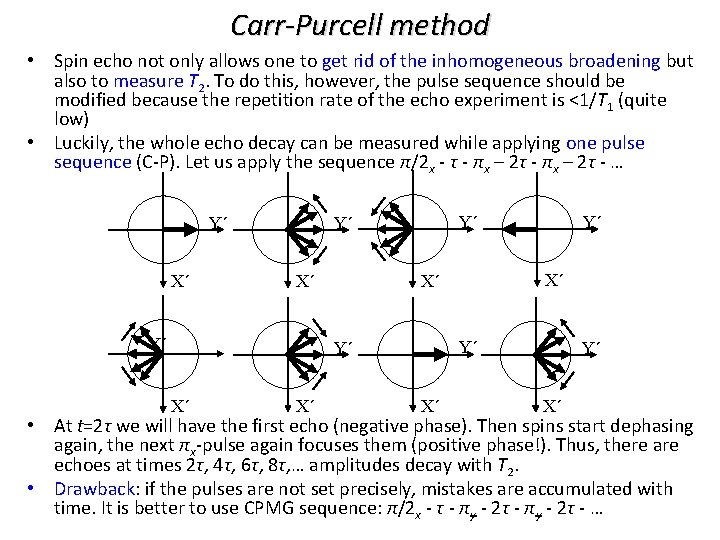
Carr-Purcell method • Spin echo not only allows one to get rid of the inhomogeneous broadening but also to measure T 2. To do this, however, the pulse sequence should be modified because the repetition rate of the echo experiment is <1/T 1 (quite low) • Luckily, the whole echo decay can be measured while applying one pulse sequence (C-P). Let us apply the sequence π/2 x - τ - πx – 2τ - … Y´ X´ Y´ Y´ Y´ X´ X´ X´ Y´ X´ • At t=2τ we will have the first echo (negative phase). Then spins start dephasing again, the next πx-pulse again focuses them (positive phase!). Thus, there are echoes at times 2τ, 4τ, 6τ, 8τ, … amplitudes decay with T 2. • Drawback: if the pulses are not set precisely, mistakes are accumulated with time. It is better to use CPMG sequence: π/2 x - τ - πy - 2τ - …

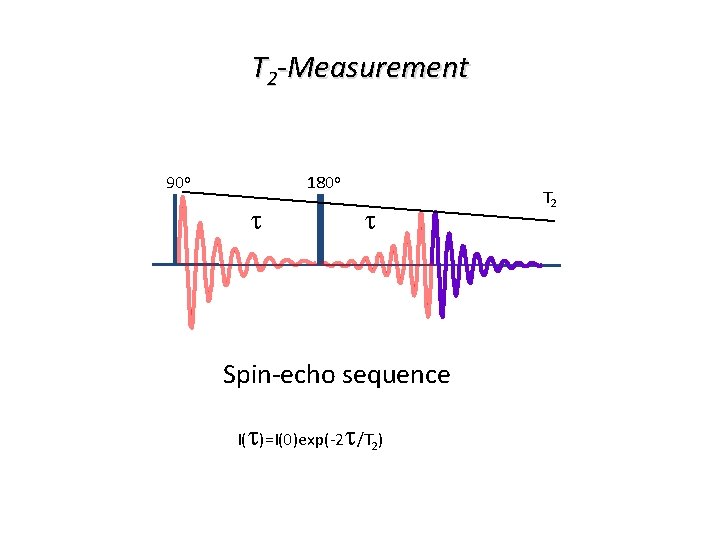
T 2 -Measurement 90 o 180 o t t Spin-echo sequence I(t)=I(0)exp(-2 t/T 2) T 2

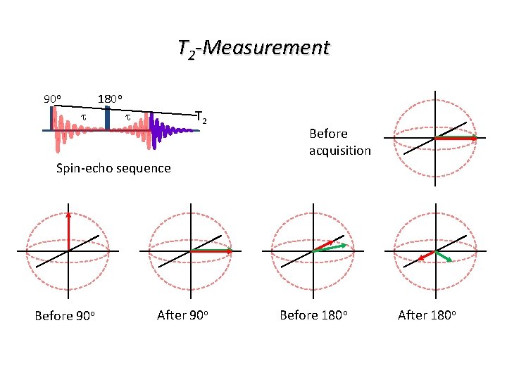
T 2 -Measurement 90 o 180 o t T 2 t Before acquisition Spin-echo sequence Before 90 o After 90 o Before 180 o After 180 o

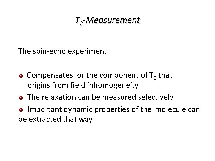
T 2 -Measurement The spin-echo experiment: Compensates for the component of T 2 that origins from field inhomogeneity The relaxation can be measured selectively Important dynamic properties of the molecule can be extracted that way

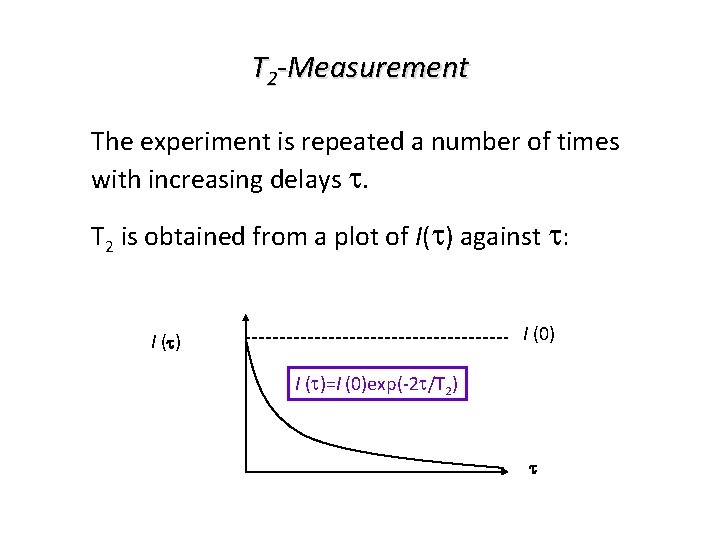
T 2 -Measurement The experiment is repeated a number of times with increasing delays t. T 2 is obtained from a plot of I(t) against t: I (0) I (t)=I (0)exp(-2 t/T 2) t

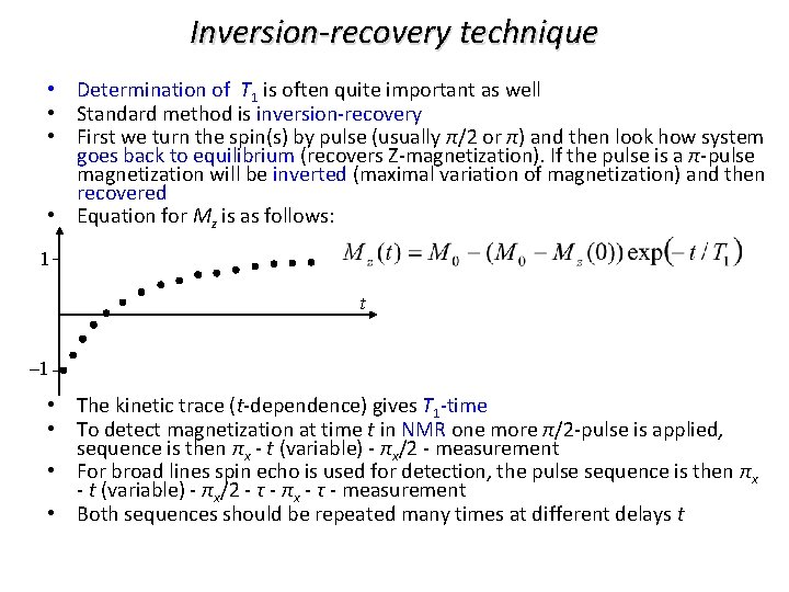
Inversion-recovery technique • Determination of T 1 is often quite important as well • Standard method is inversion-recovery • First we turn the spin(s) by pulse (usually π/2 or π) and then look how system goes back to equilibrium (recovers Z-magnetization). If the pulse is a π-pulse magnetization will be inverted (maximal variation of magnetization) and then recovered • Equation for Mz is as follows: 1 t – 1 • The kinetic trace (t-dependence) gives T 1 -time • To detect magnetization at time t in NMR one more π/2 -pulse is applied, sequence is then πx - t (variable) - πx/2 - measurement • For broad lines spin echo is used for detection, the pulse sequence is then πx - t (variable) - πx/2 - τ - πx - τ - measurement • Both sequences should be repeated many times at different delays t

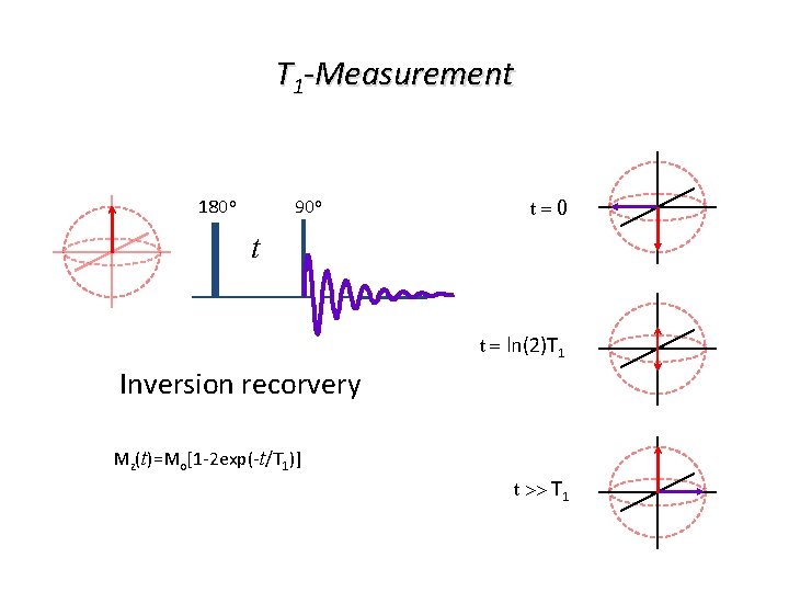
T 1 -Measurement 180 o 90 o t=0 t t = ln(2)T 1 Inversion recorvery Mz(t)=Mo[1 -2 exp(-t/T 1)] t >> T 1

Inversion-Recovery t Mz(t)=Mo[1 -2 exp(-t/T 1)]

Inversion-Recovery Mz +1 t 0 -1 t = ln(2)T 1 Mz(t)=Mo[1 -2 exp(-t/T 1)] t >> T 1

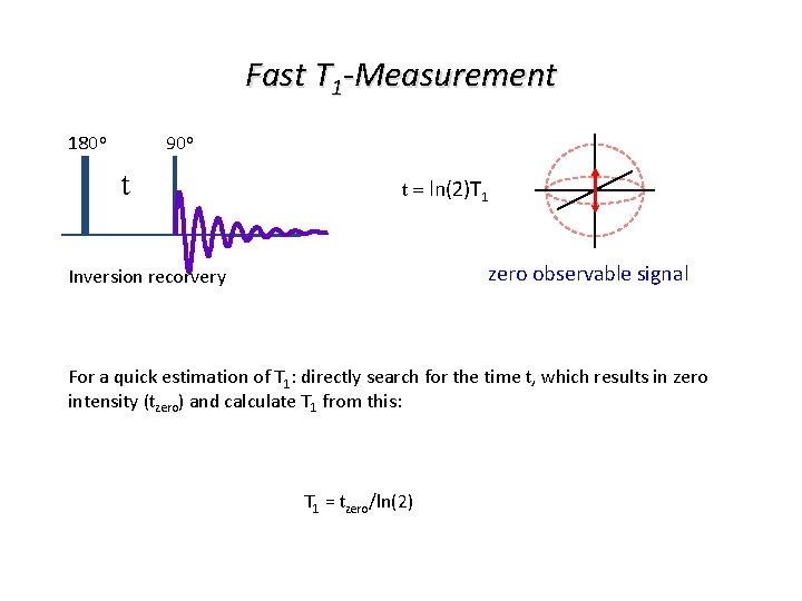
Fast T 1 -Measurement 180 o 90 o t t = ln(2)T 1 zero observable signal Inversion recorvery For a quick estimation of T 1: directly search for the time t, which results in zero intensity (tzero) and calculate T 1 from this: T 1 = tzero/ln(2)

NMR: NMR spectrometer

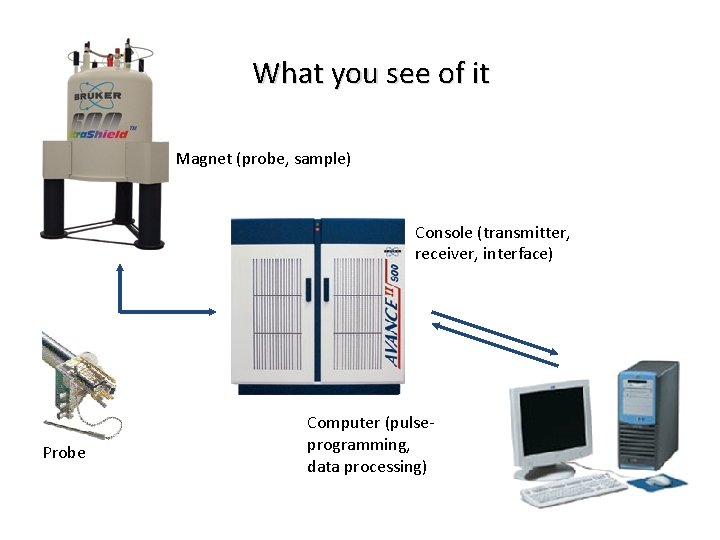
What you see of it Magnet (probe, sample) Console (transmitter, receiver, interface) Probe Computer (pulseprogramming, data processing)

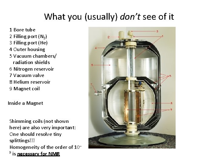
What you (usually) don’t see of it 1 Bore tube 2 Filling port (N 2) 3 Filling port (He) 4 Outer housing 5 Vacuum chambers/ radiation shields 6 Nitrogen reservoir 7 Vacuum valve 8 Helium reservoir 9 Magnet coil Inside a Magnet Shimming coils (not shown here) are also very important: One should resolve tiny splittings!!! Homogeneity of the order of 10– 9 is necessary for NMR

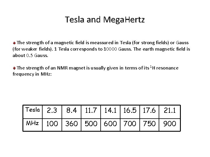
Tesla and Mega. Hertz The strength of a magnetic field is meassured in Tesla (for strong fields) or Gauss (for weaker fields). 1 Tesla corresponds to 10000 Gauss. The earth magnetic field is about 0. 5 Gauss. The strength of an NMR magnet is usually given in terms of its 1 H resonance frequency in MHz: Tesla 2. 3 8. 4 11. 7 14. 1 16. 5 17. 6 21. 1 MHz 100 360 500 600 750 900

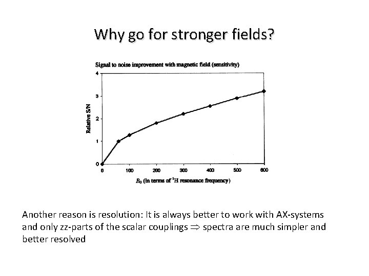
Why go for stronger fields? Another reason is resolution: It is always better to work with AX-systems and only zz-parts of the scalar couplings spectra are much simpler and better resolved

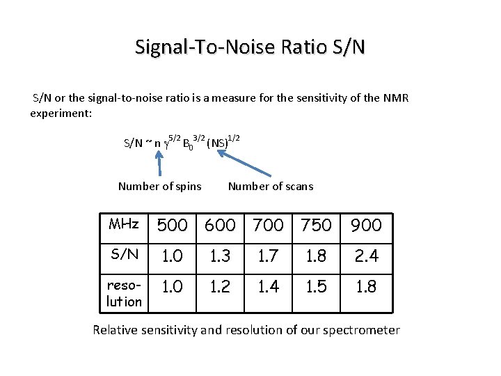
Signal-To-Noise Ratio S/N or the signal-to-noise ratio is a measure for the sensitivity of the NMR experiment: S/N ~ n g 5/2 B 03/2 (NS)1/2 Number of spins Number of scans MHz 500 600 750 900 S/N 1. 0 1. 3 1. 7 1. 8 2. 4 resolution 1. 0 1. 2 1. 4 1. 5 1. 8 Relative sensitivity and resolution of our spectrometer

NMR probe Locates the sample at homogeneous field; RF curcuit and coil for irradiating the sample and detecting its subsequent response; Additional functions (sample rotations, T stabilization, field gradients)

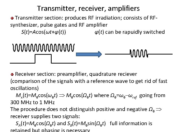
Transmitter, receiver, amplifiers Transmitter section: produces RF irradiation; consists of RFsynthesizer, pulse gates and RF amplifier S(t)=Acos(ωt+φ(t)) φ(t) can be rapuidly switched Receiver section: preamplifier, quadrature reciever (comparison of the signals with a reference wave to get rid of fast oscillations) Mx(t)=M 0 cos(ω0 t) M 0 cos(Ω 0 t) where Ω 0=ω0–ωref going from 300 MHz to 1 MHz The procedure does not distinguish positive and negative Ω 0 receiver supplies two signals: SA(t)=M 0 cos(Ω 0 t) and SB(t)=M 0 sin(Ω 0 t) full information is

Hardware (Summary) Magnet (Dewar, coil, shims) Probe Transmitter, receiver, amplifiers Acquisition computer (ADC) Sensitivity

NMR: NOE

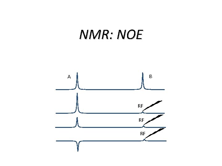
NMR: NOE=Nuclear Overhauser Effect Overhauser effect (EPR and NMR meet): NMR enhancement after pumping EPR transitions; works on dipolar relaxation of electron and nucleus NOE also works using dipolar relaxation of two nuclei Applications are quite different: not mainly enhancing NMR signals but rather measuring distances between spins

NMR: NOE B A RF RF RF

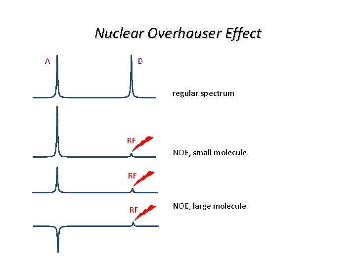
Nuclear Overhauser Effect B A regular spectrum RF NOE, small molecule RF RF NOE, large molecule

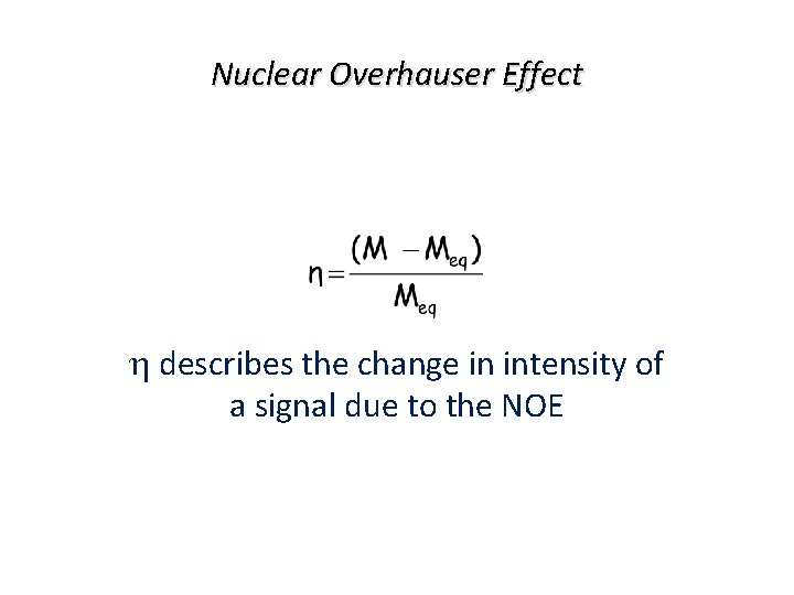
Nuclear Overhauser Effect describes the change in intensity of a signal due to the NOE

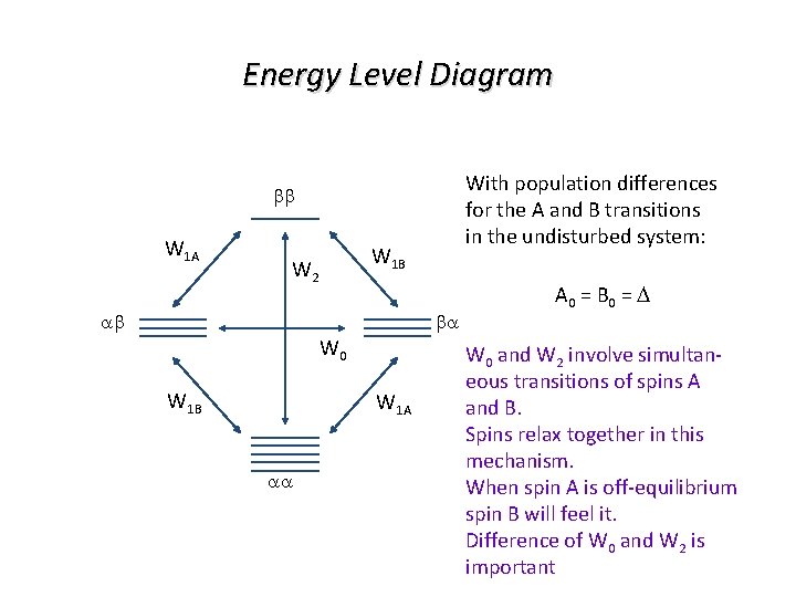
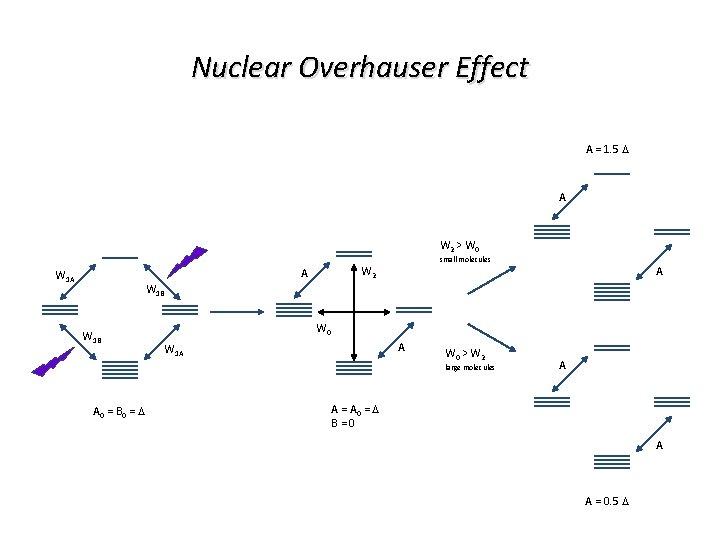
Energy Level Diagram With population differences for the A and B transitions in the undisturbed system: bb W 1 A W 1 B W 2 ab ba W 0 W 1 B W 1 A aa A 0 = B 0 = D W 0 and W 2 involve simultaneous transitions of spins A and B. Spins relax together in this mechanism. When spin A is off-equilibrium spin B will feel it. Difference of W 0 and W 2 is important

Nuclear Overhauser Effect A = 1. 5 D A W 2 > W 0 A W 1 A small molecules W 2 A W 1 B W 0 A W 1 A W 0 > W 2 large molecules A 0 = B 0 = D A A = A 0 = D B = 0 A A = 0. 5 D

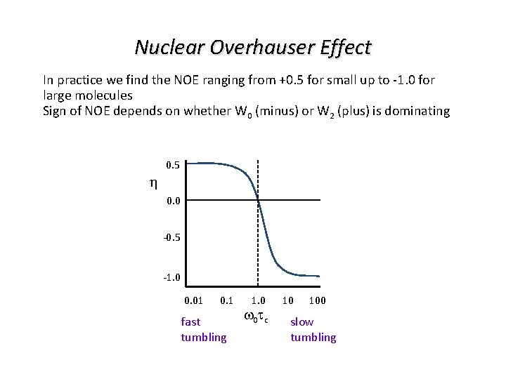
Nuclear Overhauser Effect In practice we find the NOE ranging from +0. 5 for small up to -1. 0 for large molecules Sign of NOE depends on whether W 0 (minus) or W 2 (plus) is dominating 0. 5 0. 0 -0. 5 -1. 0 0. 01 0. 1 fast tumbling 1. 0 w 0 t c 10 100 slow tumbling

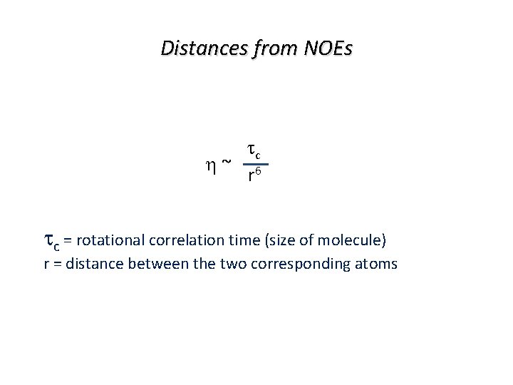
Distances from NOEs tc ~ 6 r tc = rotational correlation time (size of molecule) r = distance between the two corresponding atoms

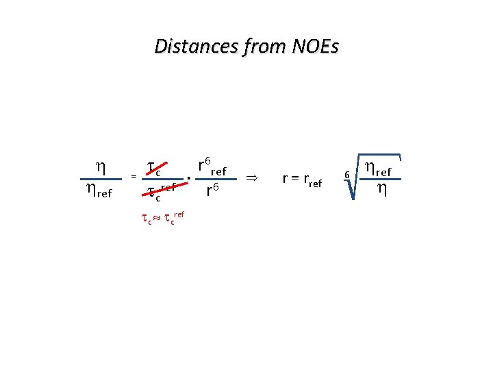
Distances from NOEs ref = tc. r 6 ref r 6 tcref tc tcref r = rref 6 ref

Application for NOEs • Information about short 1 H-1 H-distances in molecules (< 5Å) • Translated into distance-constraints applied in Molecular Simulations • Main source of structural information in NMR

Application for NOEs • Information about short 1 H-1 H-distances in molecules (< 5Å) • Translated into distance-constraints applied in Molecular Simulations • Main source of structural information in NMR • It will be explained how it works

NMR: 2 D-NMR

NMR: 2 D-NMR Why is 1 D (just NMR spectrum) not enough?

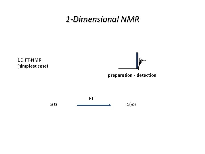
1 -Dimensional NMR 1 D FT-NMR (simplest case) preparation - detection S(t) FT S(w)

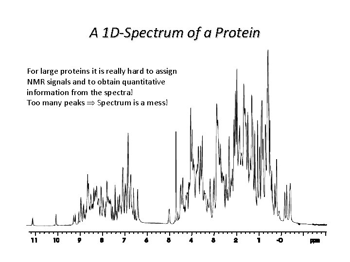
A 1 D-Spectrum of a Protein For large proteins it is really hard to assign NMR signals and to obtain quantitative information from the spectra! Too many peaks Spectrum is a mess!

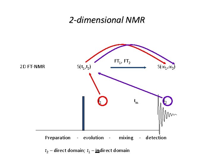
2 -dimensional NMR 2 D FT-NMR FT 1, FT 2 S(t 1, t 2) t 1 S(w 1, w 2) tm t 2 Preparation - evolution - mixing - detection t 2 – direct domain; t 1 – indirect domain

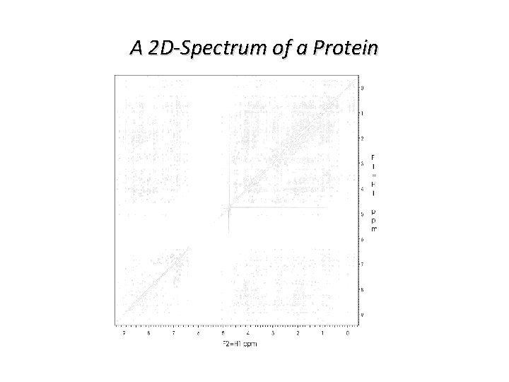
A 2 D-Spectrum of a Protein

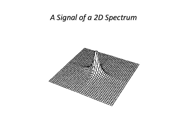
A Signal of a 2 D Spectrum

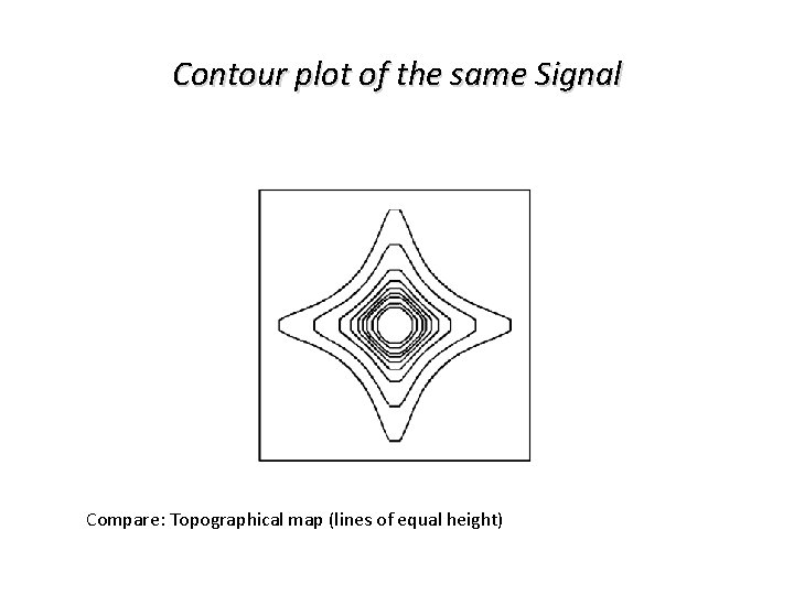
Contour plot of the same Signal Compare: Topographical map (lines of equal height)

Now let us see how it works How to get to this second dimension? ? ?

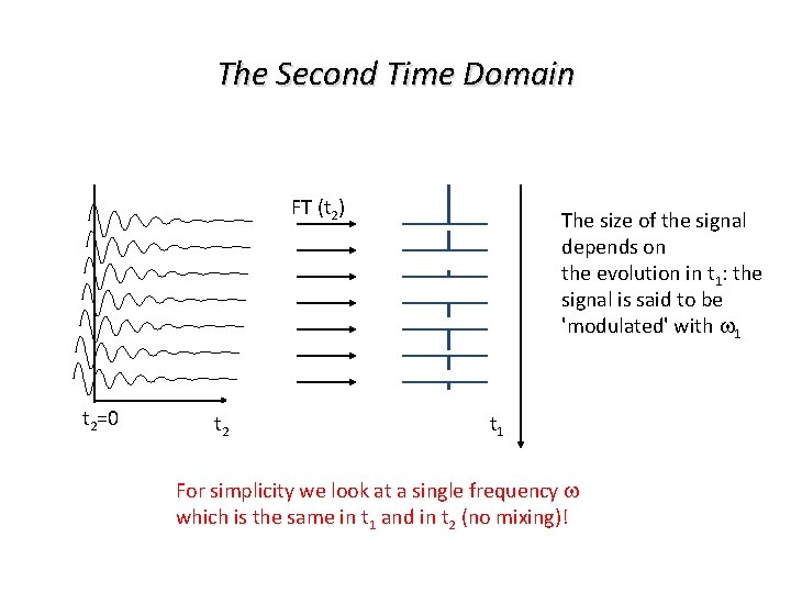
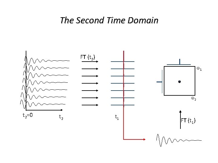
The Second Time Domain FT (t 2) t 2=0 t 2 The size of the signal depends on the evolution in t 1: the signal is said to be 'modulated' with w 1 t 1 For simplicity we look at a single frequency w which is the same in t 1 and in t 2 (no mixing)!

The Second Time Domain FT (t 2) w 1 w 2 t 2=0 t 2 t 1 FT (t 1)

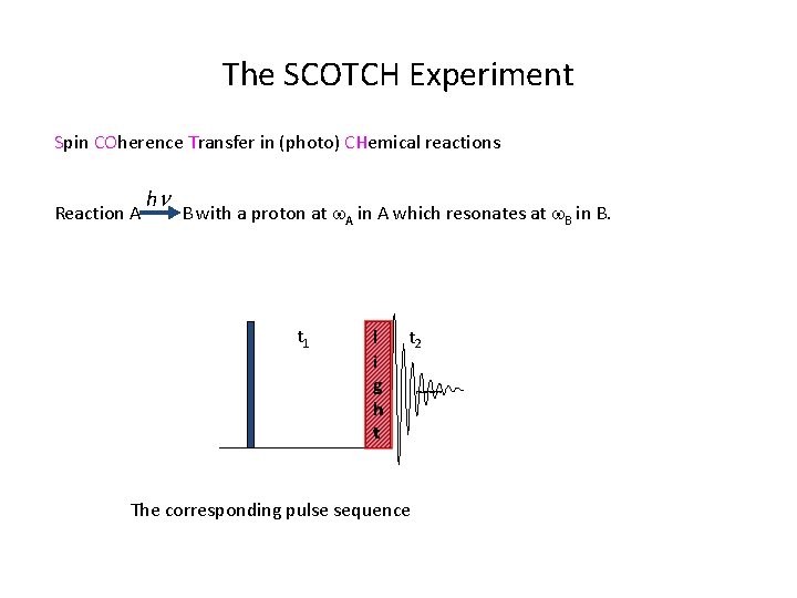
The SCOTCH Experiment Spin COherence Transfer in (photo) CHemical reactions hn Reaction A B with a proton at w. A in A which resonates at w. B in B. t 1 l i g h t t 2 The corresponding pulse sequence

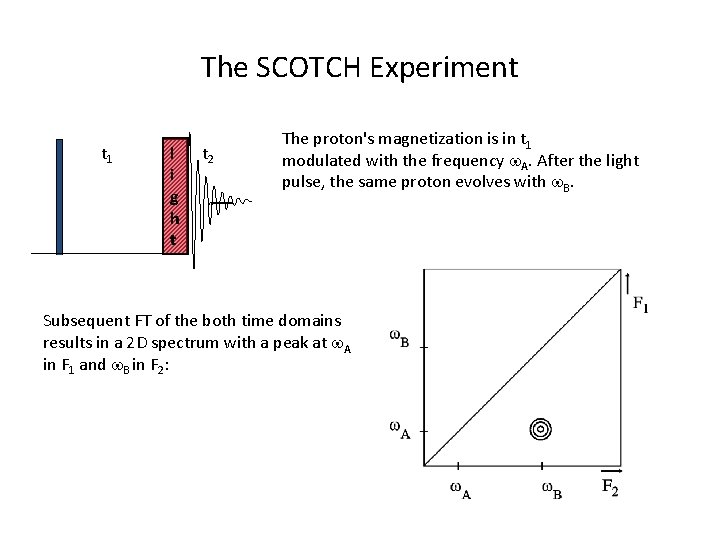
The SCOTCH Experiment t 1 l i g h t t 2 The proton's magnetization is in t 1 modulated with the frequency w. A. After the light pulse, the same proton evolves with w. B. Subsequent FT of the both time domains results in a 2 D spectrum with a peak at w. A in F 1 and w. B in F 2:

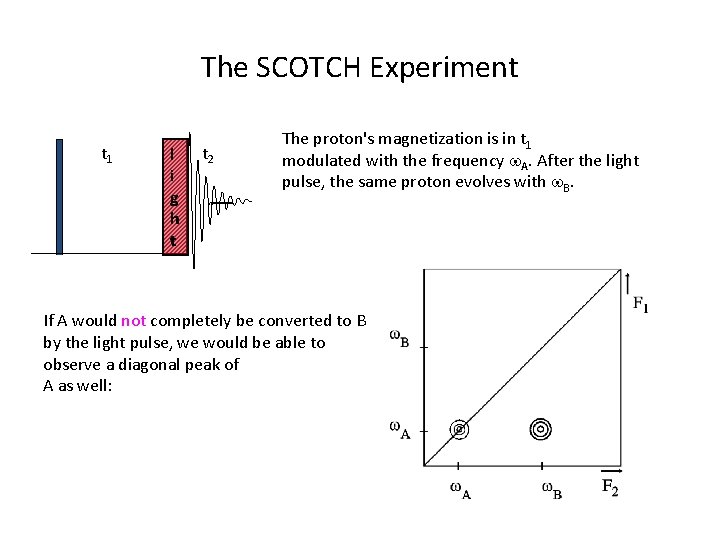
The SCOTCH Experiment t 1 l i g h t t 2 The proton's magnetization is in t 1 modulated with the frequency w. A. After the light pulse, the same proton evolves with w. B. If A would not completely be converted to B by the light pulse, we would be able to observe a diagonal peak of A as well:

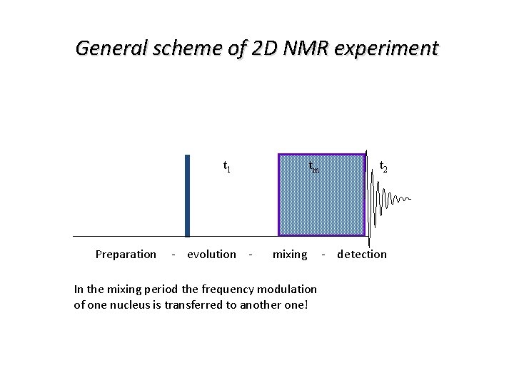
General scheme of 2 D NMR experiment t 1 tm t 2 Preparation - evolution - mixing - detection In the mixing period the frequency modulation of one nucleus is transferred to another one!

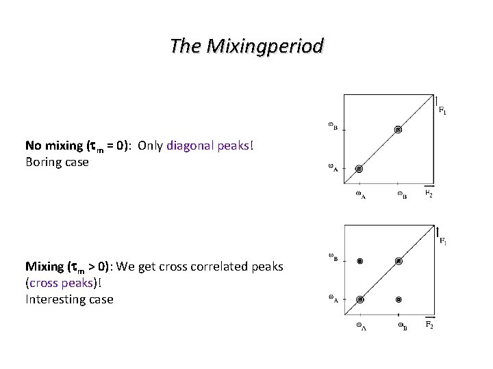
The Mixingperiod No mixing (tm = 0): Only diagonal peaks! Boring case Mixing (tm > 0): We get cross correlated peaks (cross peaks)! Interesting case

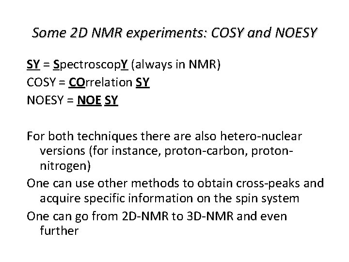
Some 2 D NMR experiments: COSY and NOESY SY = Spectroscop. Y (always in NMR) COSY = COrrelation SY NOESY = NOE SY For both techniques there also hetero-nuclear versions (for instance, proton-carbon, protonnitrogen) One can use other methods to obtain cross-peaks and acquire specific information on the spin system One can go from 2 D-NMR to 3 D-NMR and even further

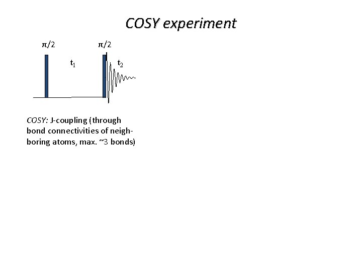
COSY experiment π/2 π/2 t 1 t 2 COSY: J-coupling (through bond connectivities of neighboring atoms, max. ~3 bonds)

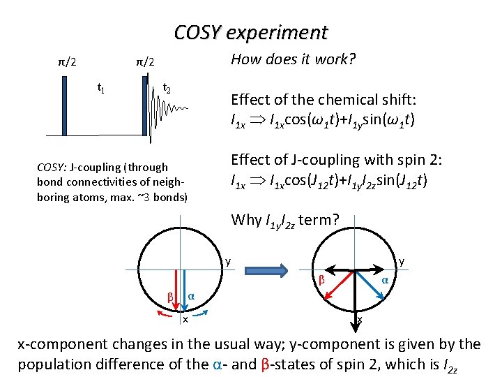
COSY experiment How does it work? π/2 π/2 t 1 t 2 Effect of the chemical shift: I 1 xcos(ω1 t)+I 1 ysin(ω1 t) COSY: J-coupling (through bond connectivities of neighboring atoms, max. ~3 bonds) Effect of J-coupling with spin 2: I 1 xcos(J 12 t)+I 1 y. I 2 zsin(J 12 t) Why I 1 y. I 2 z term? y y β β α α x x x-component changes in the usual way; y-component is given by the population difference of the α- and β-states of spin 2, which is I 2 z

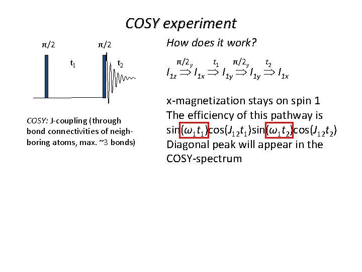
COSY experiment How does it work? π/2 π/2 t 1 t 2 COSY: J-coupling (through bond connectivities of neighboring atoms, max. ~3 bonds) π/2 y t 1 π/2 y t 2 I 1 z I 1 x I 1 y I 1 x x-magnetization stays on spin 1 The efficiency of this pathway is sin(ω1 t 1)cos(J 12 t 1)sin(ω1 t 2)cos(J 12 t 2) Diagonal peak will appear in the COSY-spectrum

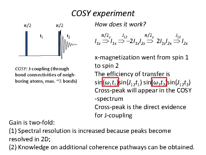
COSY experiment How does it work? π/2 π/2 t 1 t 2 COSY: J-coupling (through bond connectivities of neighboring atoms, max. ~3 bonds) π/2 y J 12 π/2 y J 12 I 1 z I 1 x – 2 I 1 x. I 2 z 2 I 1 z. I 2 x x-magnetization went from spin 1 to spin 2 The efficiency of transfer is sin(ω1 t 1)sin(J 12 t 1) sin(ω2 t 2)sin(J 12 t 2) Cross-peak will appear in the COSY -spectrum Cross-peak is the direct evidence for J-coupling Gain is two-fold: (1) Spectral resolution is increased because peaks become resolved in 2 D; (2) Knowledge on additional coherence pathways can be obtained.

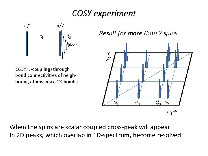
COSY experiment π/2 π/2 t 2 Result for more than 2 spins ω2 → t 1 COSY: J-coupling (through bond connectivities of neighboring atoms, max. ~3 bonds) Ω 1 Ω 2 Ω 3 Ω 4 ω1→ When the spins are scalar coupled cross-peak will appear In 2 D peaks, which overlap in 1 D-spectrum, become resolved

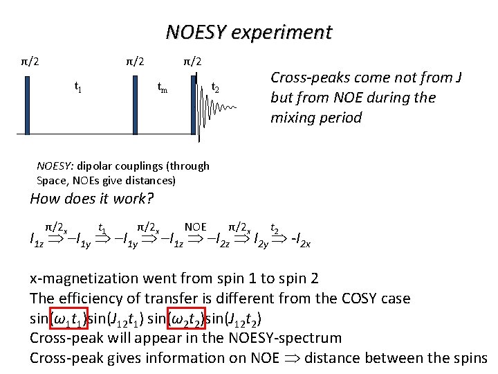
NOESY experiment π/2 π/2 t 1 tm t 2 Cross-peaks come not from J but from NOE during the mixing period NOESY: dipolar couplings (through Space, NOEs give distances) How does it work? π/2 x t 1 π/2 x NOE π/2 x t 2 I 1 z –I 1 y –I 1 z –I 2 z I 2 y -I 2 x x-magnetization went from spin 1 to spin 2 The efficiency of transfer is different from the COSY case sin(ω1 t 1)sin(J 12 t 1) sin(ω2 t 2)sin(J 12 t 2) Cross-peak will appear in the NOESY-spectrum Cross-peak gives information on NOE distance between the spins

Some 2 D NMR experiments: COSY and NOESY SY = Spectroscop. Y (always in NMR) COSY = COrrelation SY NOESY = NOE SY For both techniques there also hetero-nuclear versions (for instance, proton-carbon, protonnitrogen) One can use other methods to obtain cross-peaks and acquire specific information on the spin system One can go from 2 D-NMR to 3 D-NMR and even further

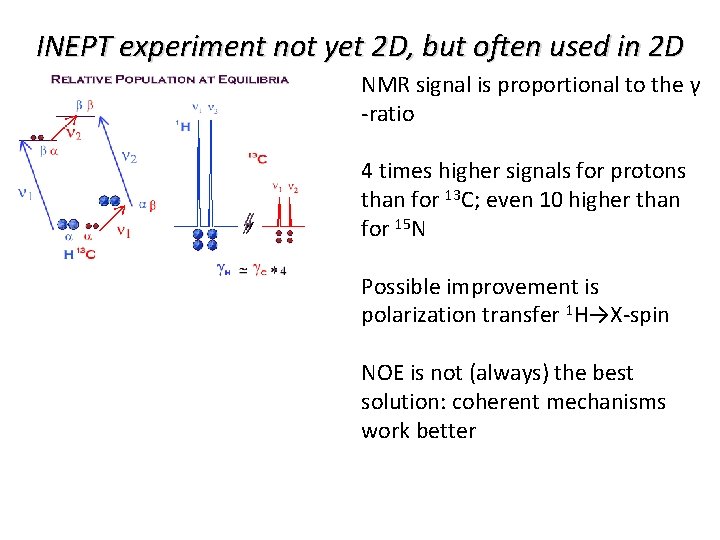
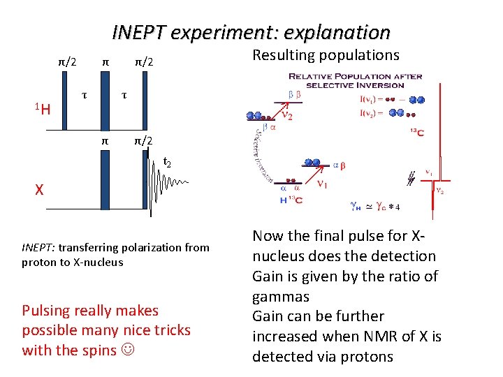
INEPT experiment not yet 2 D, but often used in 2 D NMR signal is proportional to the γ -ratio 4 times higher signals for protons than for 13 C; even 10 higher than for 15 N Possible improvement is polarization transfer 1 H→X-spin NOE is not (always) the best solution: coherent mechanisms work better

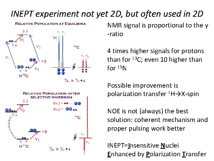
INEPT experiment not yet 2 D, but often used in 2 D NMR signal is proportional to the γ -ratio 4 times higher signals for protons than for 13 C; even 10 higher than for 15 N Possible improvement is polarization transfer 1 H→X-spin NOE is not (always) the best solution: coherent mechanism and proper pulsing work better INEPT=Insensitive Nuclei Enhanced by Polarization Transfer

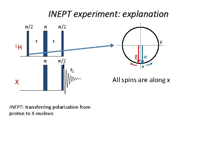
INEPT experiment: explanation π/2 1 H τ τ y β π/2 t 2 X INEPT: transferring polarization from proton to X-nucleus α x All spins are along x

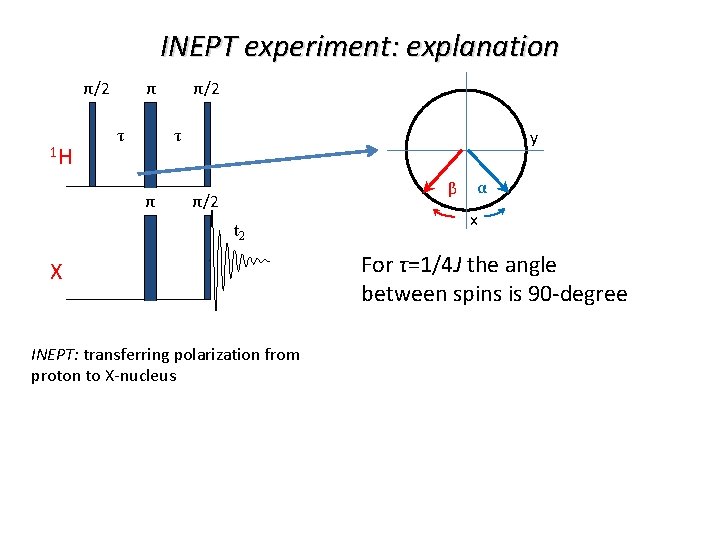
INEPT experiment: explanation π/2 1 H τ τ y β π/2 t 2 X INEPT: transferring polarization from proton to X-nucleus α x For τ=1/4 J the angle between spins is 90 -degree

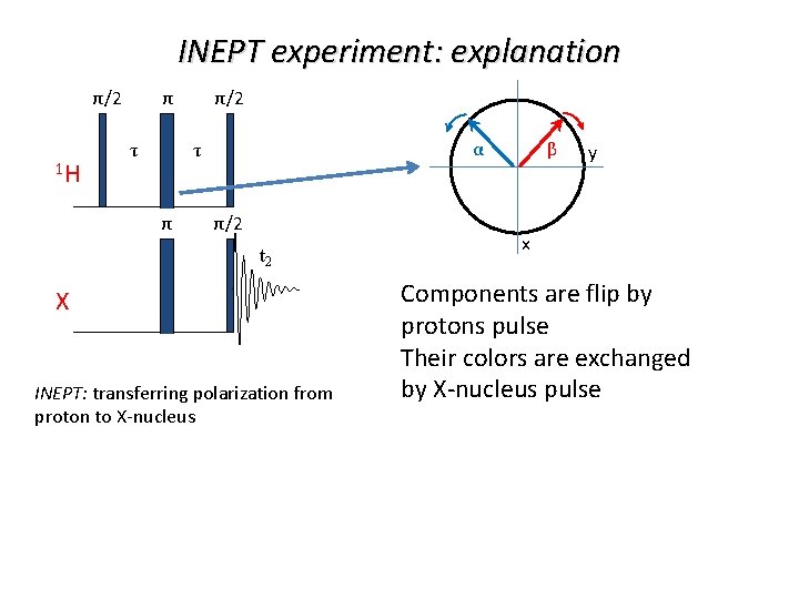
INEPT experiment: explanation π/2 1 H τ α τ π/2 t 2 X INEPT: transferring polarization from proton to X-nucleus β y x Components are flip by protons pulse Their colors are exchanged by X-nucleus pulse

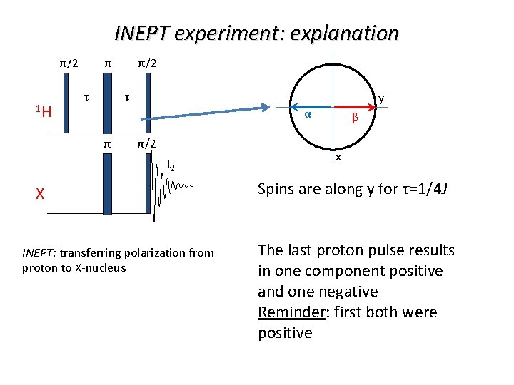
INEPT experiment: explanation π/2 1 H τ τ y α π/2 t 2 X INEPT: transferring polarization from proton to X-nucleus β x Spins are along y for τ=1/4 J The last proton pulse results in one component positive and one negative Reminder: first both were positive

INEPT experiment: explanation Resulting populations π/2 1 H τ τ π/2 t 2 X INEPT: transferring polarization from proton to X-nucleus Pulsing really makes possible many nice tricks with the spins Now the final pulse for Xnucleus does the detection Gain is given by the ratio of gammas Gain can be further increased when NMR of X is detected via protons

The rest of 2 D-NMR will be given by Prof. Robert Kaptein The rest is: (i) Other methods; (ii) Their applications to proteins.