NI Multisim Simulation Software University of New Mexico

NI Multisim Simulation Software University of New Mexico Electrical & Computer Engineering ECE 206 L, Instrumentation

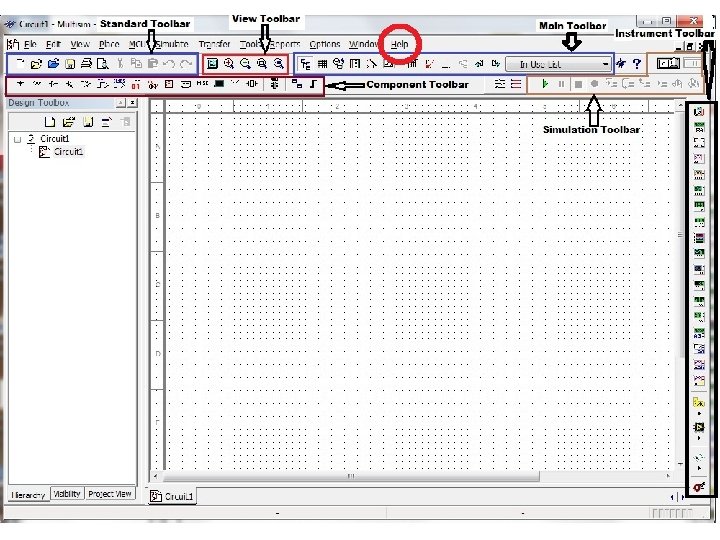
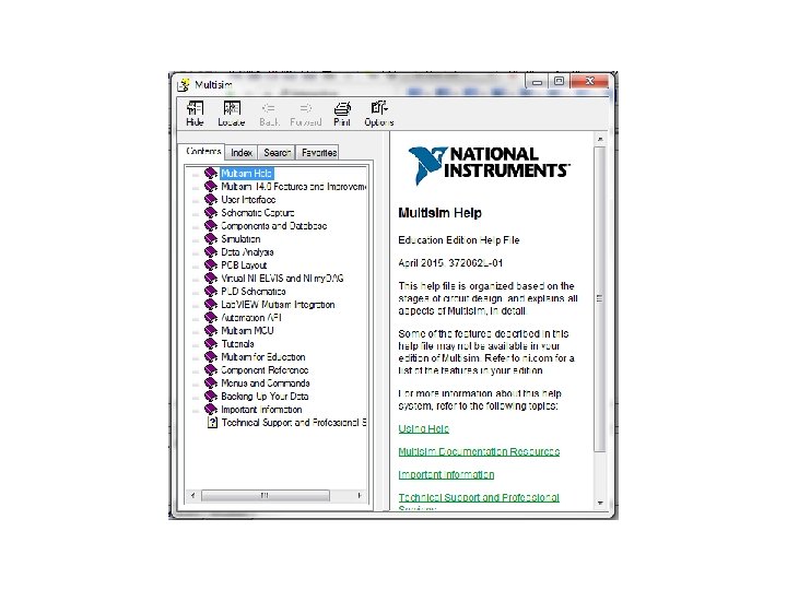
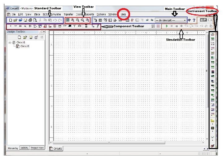
National Instruments Multisim Simulation Software • Multisim™ software integrates industrystandard SPICE simulation with an interactive schematic environment to visualize and analyze electronic circuit • The top of the GUI window contains the HELP command that brings up the Multisim Help window. • This Help window provides a comprehensive description of how to use Multisim.

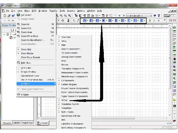
Toolbars • The toolbars can be customized to your preference from the View tool command. • View > Toolbars > then check or uncheck the tool bars you would like to have displayed. • The individual Toolbars are placed in the Toolbar area, then can be ‘floated’ within the work area. • Note the Instrument Toolbar on the right side of the circuit work area.

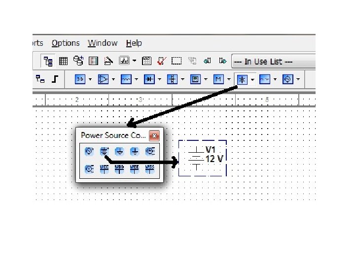
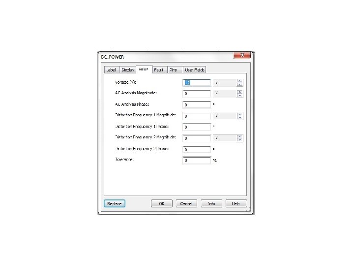
Building the First Circuit • From View command place the Virtual Toolbar on the toolbar space • From the Virtual Toolbar select the DC Power Source and place it on the work area. (next slide) • (slide after next) Double click the VI, DC Power Source and it will open the settings window where its characteristics can be adjusted. • When setting are complete, click OK

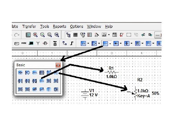
From the Basic Toolbar • Select a Resistor and if necessary set it value to 1 k. Ohms. It should default to this value. • Select a Potentiometer. Its default value should be 1 k. Ohms. • Note the Potentiometer has a percentage adjustment for where its wiper is set using the mouse. • Lastly, from the Virtual Power Source select the Ground and place it on the page.

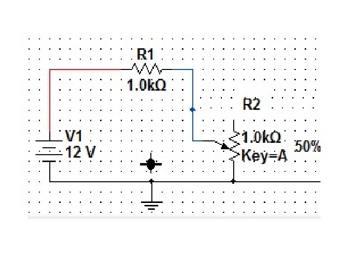
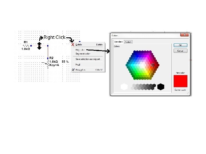
Wiring/Connecting Components • By hovering the mouse over the end of a component, the wiring action will be activated. • Left click to start the wiring and at the destination again left click to end the wire. • Hover the mouse over the wire and right click will open the wire menu. Select Net color and the Colors menu window opens for setting the color of the wire. See next 2 slide. • Connect up the circuit as shown

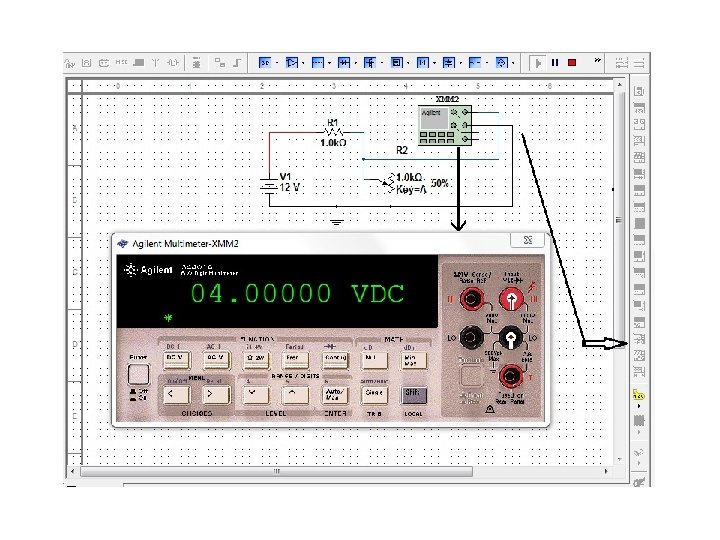
Connecting Simulated Instruments • From the Instrument Tool bar, hover the mouse over each icon to see each device and click on the Agilent DMM and place it next to the circuit. • Double click on the schematic symbol of the DMM to open its front panel. • Wire the meter to the circuit as shown in the next slide. • Click the [Power] and [DC V] buttons on the meter. • Digital Multimeters values are in rms units.

Making a Measurement • Under the Simulate drop down menu select RUN. • Using the mouse, change the wiper’s percentage setting on the Potentiometer and see the voltage reading change. At 50% it should read 4 Vdc and at 100%, 6 Vdc. • Under Simulate click stop. • If the Simulation toolbar is viewed, then you can use the green, play, and red, stop, buttons

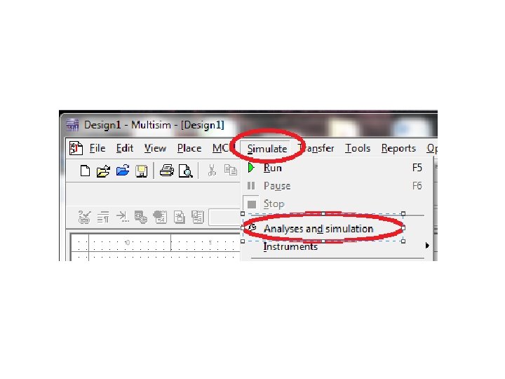
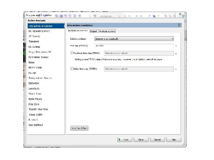
Circuit Analysis • Under Simulate > Analysis and Simulation selection will open the Analysis Window for configuring various circuit analysis routines, including: – DC Operation Point – Transient – Parameter Sweep – Fourier – Distortion – Worst Case - AC Sweep - DC Sweep - Noise - Temperature Sweep - Pole Zero - Other

Circuit Probes • From Simulation > Probe Settings, probes can be place at various circuit points to provide measurements during simulation.

Multisim Lab Considerations Analysis of DC Circuit & AC Circuit

Calculating Loop Currents & Component Voltages • The Lab Procedure is to simulate a DC circuit and an AC circuit. • A circuit (or subcircuit) is in series if the path through the circuit passes through each component before pass through the next. • A circuit (or subcircuit) is in parallel if the path through the circuit can be through more than one component at a time. •

Loop Currents, Component Voltages • Ohm’s Law: Voltage = Current times Impedance • Kirchhoff’s Voltage Law, KVL: The sum of voltages around a closed electrical loop is zero. • Kirchhoff’s Current Law, KCL: The algebraic sum of the currents at a node is zero. • The total impedance of impedances in series is the sum of impedances. • The total impedance of impedances in parallel is:

Consider the Lab’s Circuits

Lab Circuit ‘a’ • This is a DC, Direct Current, Circuit meaning the current never reverses flow direction. • There are two loops and two loop currents: I 1, I 2 • There are four Component Voltages: VR 1, VR 2, VR 3, & VI 1 • The sum of voltages around Loop 2: VR 1+VR 2+VR 3=0 • The loop current value is the value of a component’s current if that component is in only 1 loop so I 1 = 4 A. • VR 1=I 2 x. R 1, VR 2=I 2 x. R 2, VR 3=R 3 x(I 2 -I 1) and using known values in the equations and substituting into Loop 2 Voltage equation above: I 2 x. R 1+I 2 R 2+R 3(I 2 -I 1) => I 2 x( R 1 + R 2 + R 3) = 4 R 3 so: I 2(4+1+5)=4 x 5 => I 2= 20/10 = 2 Amps • I 1=4 A, I 2=2 A, VR 1=8 V, VR 2=2 V, VR 3=VI 1=10 V • Perform the Simulation and see if the results are the same.

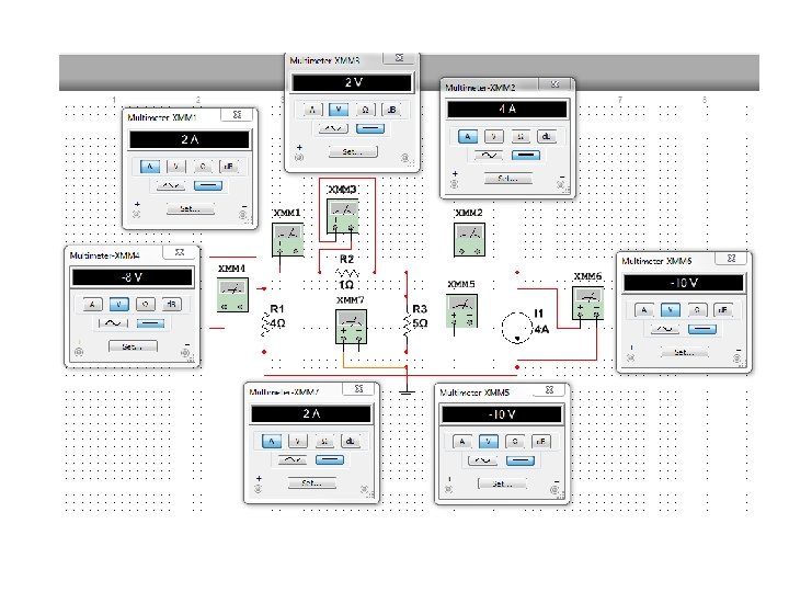
Lab Circuit ‘a’ Simulation • Digital Multi. Meters, XMM 1, XMM 2, & XMM 7 measure current and the ‘A’ button , and DC button are highlighted. • Note that the wire connecting R 1 to R 2 must be broken and the DMM, XMM 1, is inserted serially into the circuit so current will flow through the meter to allow measurement of the current. • XMM 1, measures Loop 2 Current, I 2, at 2 Amps • XMM 2 measures Loop 1 Current, I 1, at 4 Amps • XMM 7 measures the current in R 3, IR 3, at (I 1 -12) = 4 -2= 2 A • All the other DMMs measure Voltage and the ‘V’ button and the DC button are highlighted. • Also note that the Voltage measurement has the meter connected in Parallel with the component to measure the voltage across the component. • XMM 3 measures VR 2 = -2 V, XMM 4 for VR 1 = -8 V • XMM 5 for VR 3= -10 V, XMM 6 for VI 1 = -10 V

Circuit ‘a’ Point of Interest • Note the VR 1 = -8 V, VR 2 = -2 V, VR 3 = -10 V. • KVL states the sum of voltage around a loop is 0. • Starting at ground and passing forward through R 1 from 0 V to -8 V then forward through R 2 for another -2 V to -10 Volt. As we pass backwards through R 3 from the negative side to the positive side we gain +10 V to ground and sum to 0 V. • (-8[VR 1]) + (-2[VR 2]) + (- -10[ -VR 3]) = -8 -2 - (-10) = 0

Now Consider Lab Circuit ‘b’

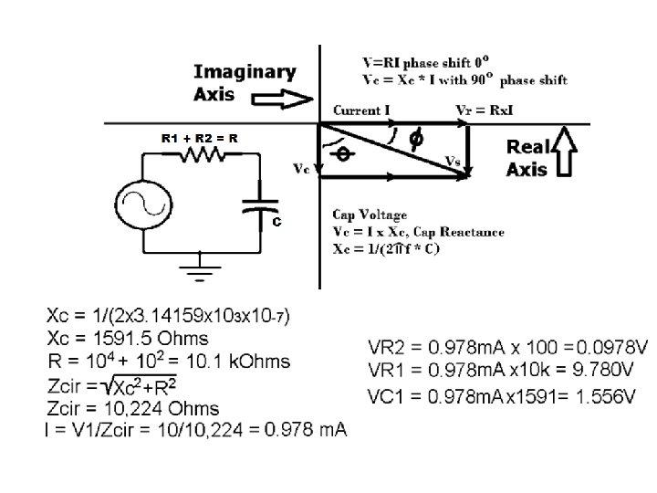
Lab Circuit b) • This is an AC (Alternating Current) Circuit with a voltage source V 1 of 10 V. Assume rms units 10 Vrms. • Need to determine the current I to calculate component voltages: VR 1, VR 2, & VC 1 • I = V 1/Zcir, where Zcir is the impedance of the circuit • Zcir will equal the sum of the impedances with a little adjustment. The capacitor voltage is 90 degrees out of phase with the capacitor current where as the resistors’ voltages are in phase with the current. • The resistor impedance must be vector summed with the capacitor impedance.

Circuit ‘b’ Point of Interest • KVL states the voltage sum around a loop is 0, but VR 1=9. 780, VR 2=0. 0978, VC 1=1. 556 and V 1=10. Now VR 1+VR 2+VC 1=V 1 if KVL is true. 9. 780+0. 0978+1. 556= 11. 4338 > 10 ? ? ? • Is KVL not true for AC circuits? NO! KVL is true • The voltage measurements are in Root Mean Squared units based on the peak voltages for sine waves. 0. 707 x Vpk = Vrms and the measurements are not aligned in time. • Remember the capacitor voltage is out of phase with the current but the resistor voltages are in phase.

Point of Interest, continued • The current is the same for both components, therefore the resistors reach peak voltage at peak current, where as, the capacitor reaches peak voltage 90 degrees later after the resistor voltage has dropped below peak. • If the instantaneous component voltages are measured at the same instant in time, then all the voltages in the loop will sum to zero and KVL will hold TRUE.

What to Remember The electrical laws, Ohms, KVL, KCL How impedances combine in Series & Parallel Know in what units you are working Know the units of the measurement instrument • Know how to connect the measurement instrument • Know how to use Multisim • •

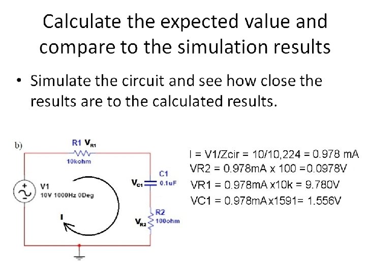
In Closing • It is best to know the approximate value of a measurement before making it. • If the measurement is significantly different from the expected value, then there exists a mistake and it should be found and corrected. • Therefore, calculate the expected values before making measurements to help catch errors.