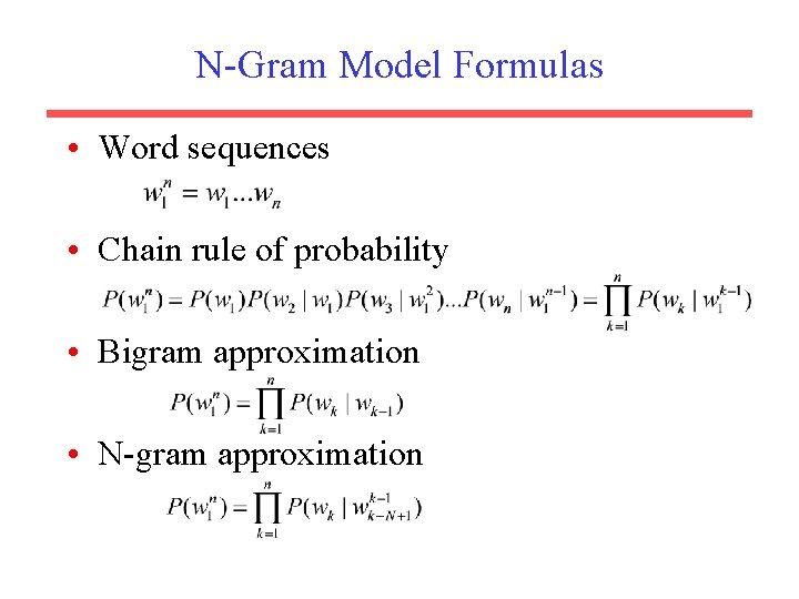
NGram Model Formulas Word sequences Chain rule of

N-Gram Model Formulas • Word sequences • Chain rule of probability • Bigram approximation • N-gram approximation

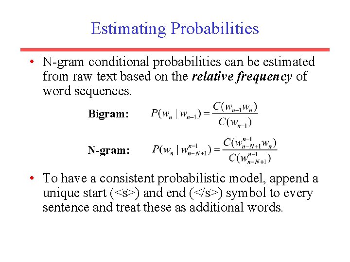
Estimating Probabilities • N-gram conditional probabilities can be estimated from raw text based on the relative frequency of word sequences. Bigram: N-gram: • To have a consistent probabilistic model, append a unique start (<s>) and end (</s>) symbol to every sentence and treat these as additional words.

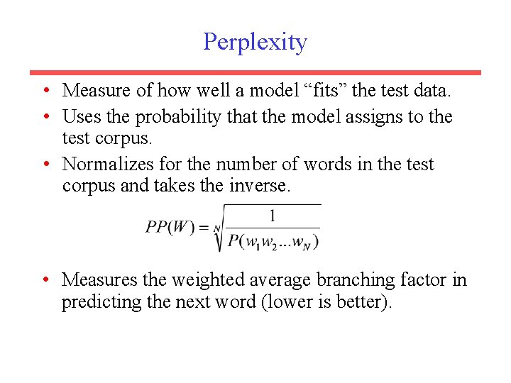
Perplexity • Measure of how well a model “fits” the test data. • Uses the probability that the model assigns to the test corpus. • Normalizes for the number of words in the test corpus and takes the inverse. • Measures the weighted average branching factor in predicting the next word (lower is better).

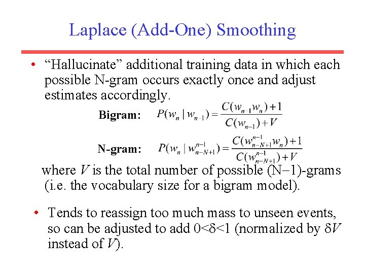
Laplace (Add-One) Smoothing • “Hallucinate” additional training data in which each possible N-gram occurs exactly once and adjust estimates accordingly. Bigram: N-gram: where V is the total number of possible (N 1)-grams (i. e. the vocabulary size for a bigram model). • Tends to reassign too much mass to unseen events, so can be adjusted to add 0< <1 (normalized by V instead of V).

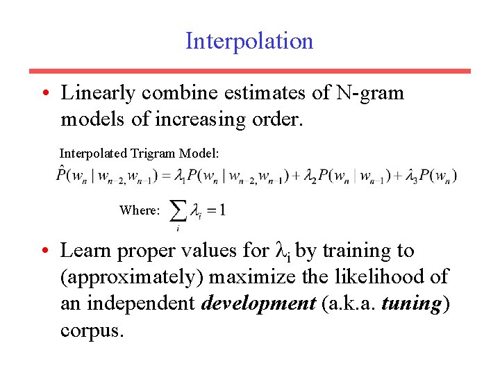
Interpolation • Linearly combine estimates of N-gram models of increasing order. Interpolated Trigram Model: Where: • Learn proper values for i by training to (approximately) maximize the likelihood of an independent development (a. k. a. tuning) corpus.

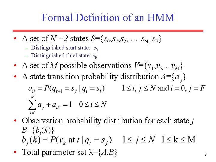
Formal Definition of an HMM • A set of N +2 states S={s 0, s 1, s 2, … s. N, s. F} – Distinguished start state: s 0 – Distinguished final state: s. F • A set of M possible observations V={v 1, v 2…v. M} • A state transition probability distribution A={aij} • Observation probability distribution for each state j B={bj(k)} • Total parameter set λ={A, B} 6

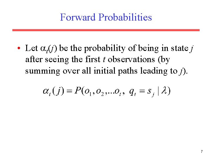
Forward Probabilities • Let t(j) be the probability of being in state j after seeing the first t observations (by summing over all initial paths leading to j). 7

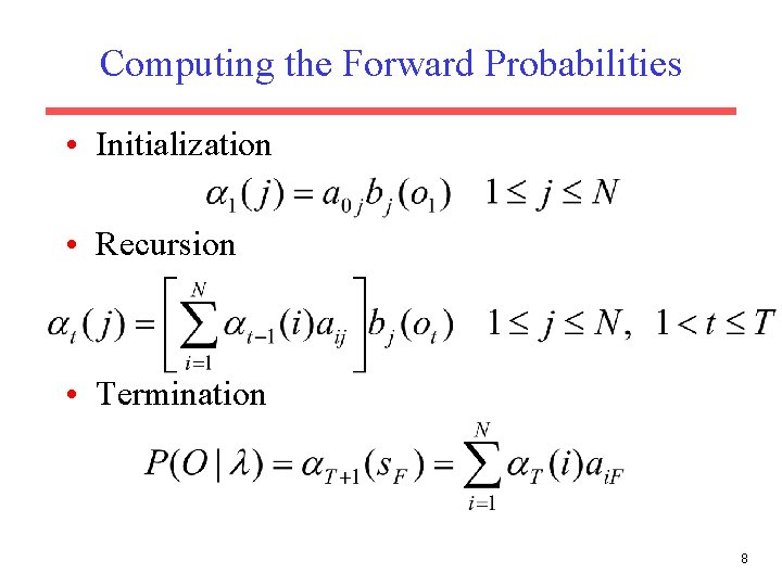
Computing the Forward Probabilities • Initialization • Recursion • Termination 8

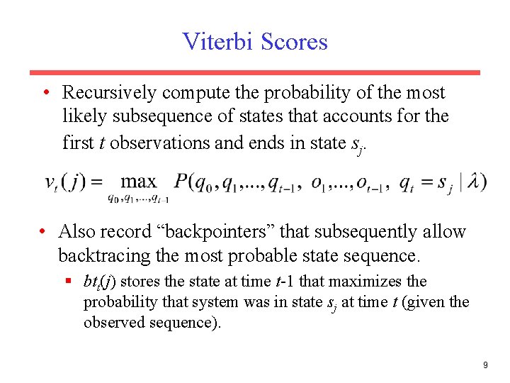
Viterbi Scores • Recursively compute the probability of the most likely subsequence of states that accounts for the first t observations and ends in state sj. • Also record “backpointers” that subsequently allow backtracing the most probable state sequence. § btt(j) stores the state at time t-1 that maximizes the probability that system was in state sj at time t (given the observed sequence). 9

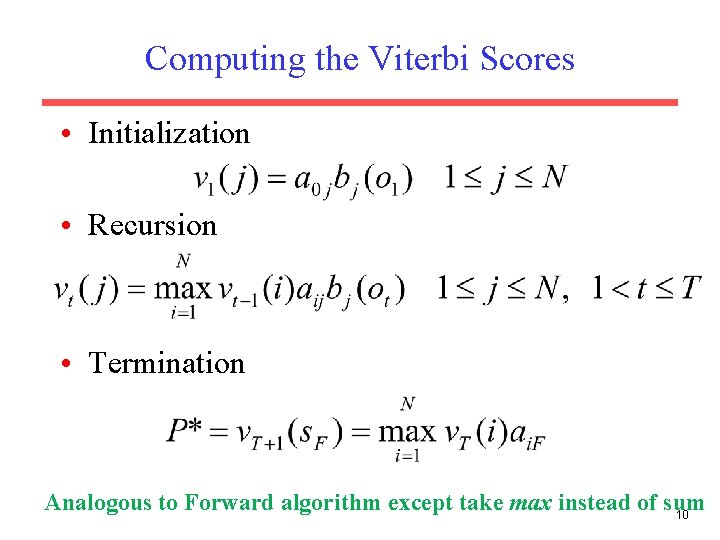
Computing the Viterbi Scores • Initialization • Recursion • Termination Analogous to Forward algorithm except take max instead of sum 10

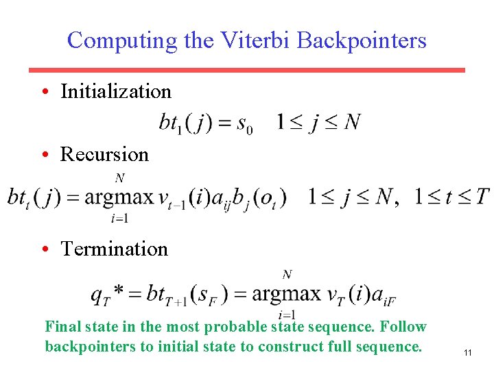
Computing the Viterbi Backpointers • Initialization • Recursion • Termination Final state in the most probable state sequence. Follow backpointers to initial state to construct full sequence. 11

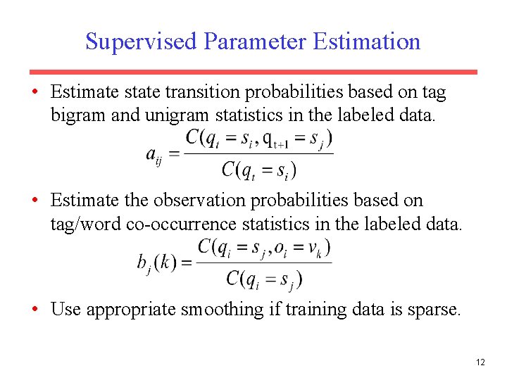
Supervised Parameter Estimation • Estimate state transition probabilities based on tag bigram and unigram statistics in the labeled data. • Estimate the observation probabilities based on tag/word co-occurrence statistics in the labeled data. • Use appropriate smoothing if training data is sparse. 12

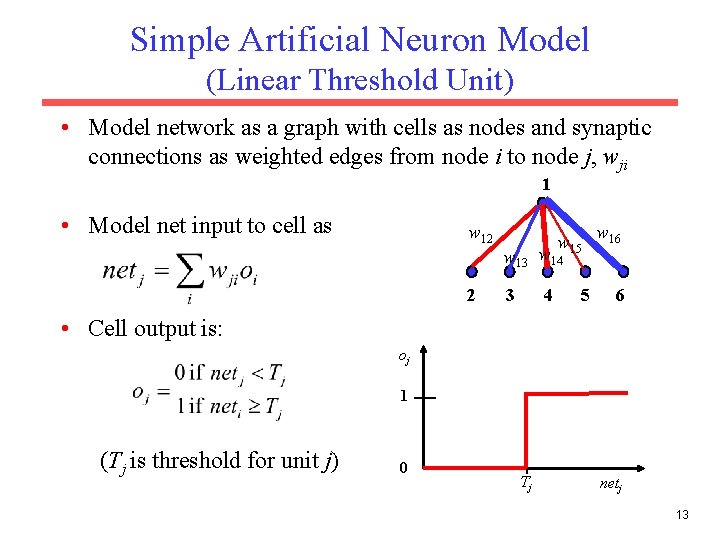
Simple Artificial Neuron Model (Linear Threshold Unit) • Model network as a graph with cells as nodes and synaptic connections as weighted edges from node i to node j, wji 1 • Model net input to cell as w 12 2 w 15 w 13 w 14 3 4 5 w 16 6 • Cell output is: oj 1 (Tj is threshold for unit j) 0 Tj netj 13

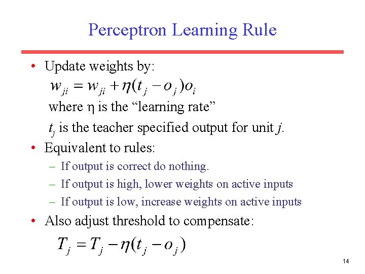
Perceptron Learning Rule • Update weights by: where η is the “learning rate” tj is the teacher specified output for unit j. • Equivalent to rules: – If output is correct do nothing. – If output is high, lower weights on active inputs – If output is low, increase weights on active inputs • Also adjust threshold to compensate: 14

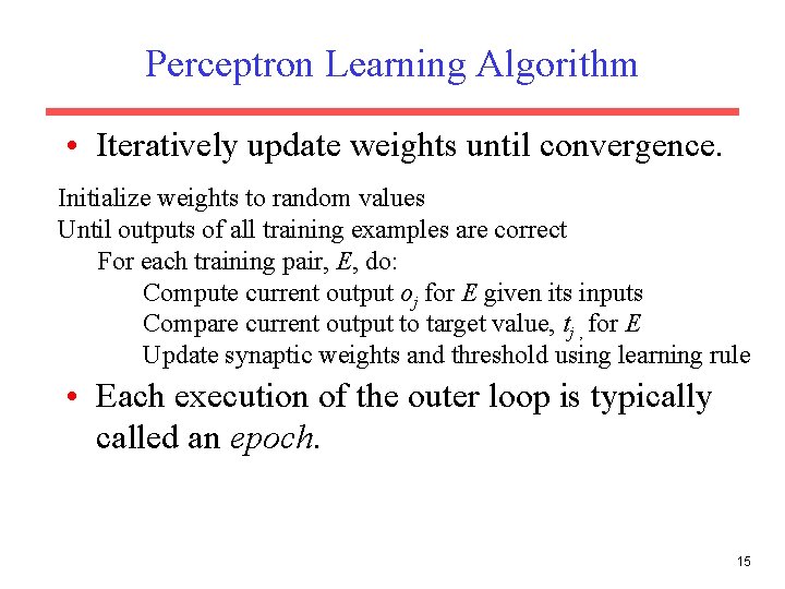
Perceptron Learning Algorithm • Iteratively update weights until convergence. Initialize weights to random values Until outputs of all training examples are correct For each training pair, E, do: Compute current output oj for E given its inputs Compare current output to target value, tj , for E Update synaptic weights and threshold using learning rule • Each execution of the outer loop is typically called an epoch. 15

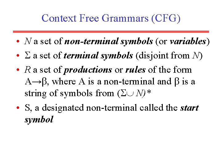
Context Free Grammars (CFG) • N a set of non-terminal symbols (or variables) • a set of terminal symbols (disjoint from N) • R a set of productions or rules of the form A→ , where A is a non-terminal and is a string of symbols from ( N)* • S, a designated non-terminal called the start symbol

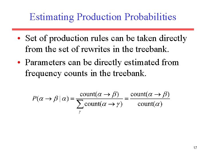
Estimating Production Probabilities • Set of production rules can be taken directly from the set of rewrites in the treebank. • Parameters can be directly estimated from frequency counts in the treebank. 17