NGram Language Models Cheng Xiang Zhai Department of

N-Gram Language Models Cheng. Xiang Zhai Department of Computer Science University of Illinois, Urbana-Champaign 1

Outline • • General questions to ask about a language model N-gram language models Special case: Unigram language models Smoothing Methods 2

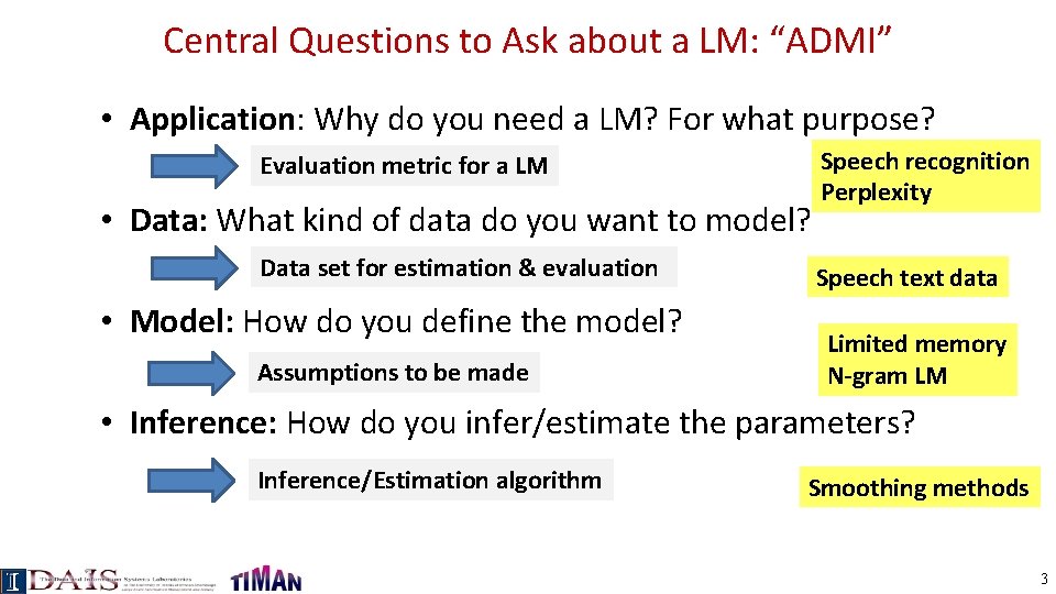
Central Questions to Ask about a LM: “ADMI” • Application: Why do you need a LM? For what purpose? Evaluation metric for a LM • Data: What kind of data do you want to model? Data set for estimation & evaluation • Model: How do you define the model? Assumptions to be made Speech recognition Perplexity Speech text data Limited memory N-gram LM • Inference: How do you infer/estimate the parameters? Inference/Estimation algorithm Smoothing methods 3

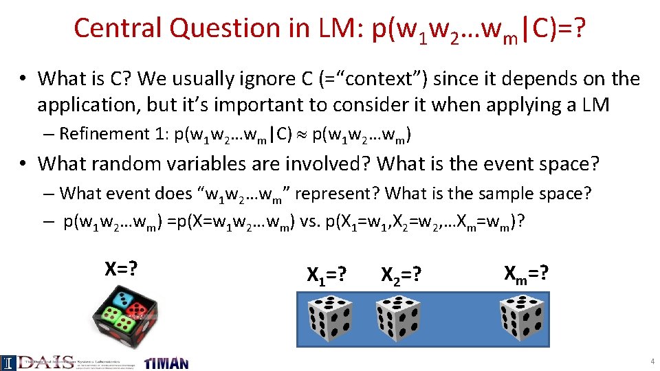
Central Question in LM: p(w 1 w 2…wm|C)=? • What is C? We usually ignore C (=“context”) since it depends on the application, but it’s important to consider it when applying a LM – Refinement 1: p(w 1 w 2…wm|C) p(w 1 w 2…wm) • What random variables are involved? What is the event space? – What event does “w 1 w 2…wm” represent? What is the sample space? – p(w 1 w 2…wm) =p(X=w 1 w 2…wm) vs. p(X 1=w 1, X 2=w 2, …Xm=wm)? X=? X 1=? X 2=? Xm=? 4

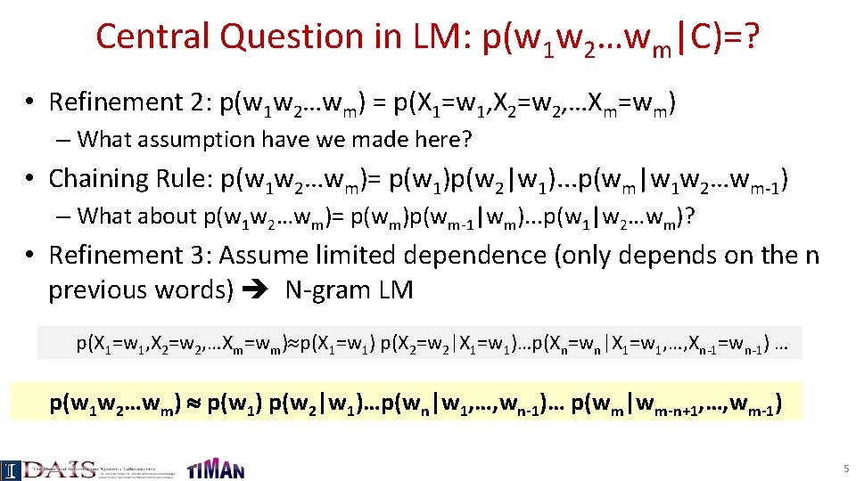
Central Question in LM: p(w 1 w 2…wm|C)=? • Refinement 2: p(w 1 w 2…wm) = p(X 1=w 1, X 2=w 2, …Xm=wm) – What assumption have we made here? • Chaining Rule: p(w 1 w 2…wm)= p(w 1)p(w 2|w 1). . . p(wm|w 1 w 2…wm-1) – What about p(w 1 w 2…wm)= p(wm)p(wm-1|wm). . . p(w 1|w 2…wm)? • Refinement 3: Assume limited dependence (only depends on the n previous words) N-gram LM p(X 1=w 1, X 2=w 2, …Xm=wm) p(X 1=w 1) p(X 2=w 2|X 1=w 1)…p(Xn=wn|X 1=w 1, …, Xn-1=wn-1) … p(w 1 w 2…wm) p(w 1) p(w 2|w 1)…p(wn|w 1, …, wn-1)… p(wm|wm-n+1, …, wm-1) 5

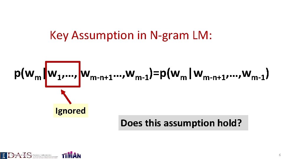
Key Assumption in N-gram LM: p(wm|w 1, …, wm-n+1…, wm-1)=p(wm|wm-n+1, …, wm-1) Ignored Does this assumption hold? 6

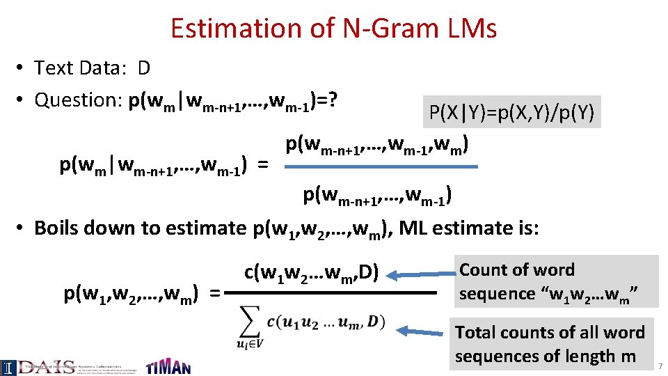
Estimation of N-Gram LMs • Text Data: D • Question: p(wm|wm-n+1, …, wm-1)=? p(wm|wm-n+1, …, wm-1) = P(X|Y)=p(X, Y)/p(Y) p(wm-n+1, …, wm-1, wm) p(wm-n+1, …, wm-1) • Boils down to estimate p(w 1, w 2, …, wm), ML estimate is: p(w 1, w 2, …, wm) = c(w 1 w 2…wm, D) Count of word sequence “w 1 w 2…wm” Total counts of all word sequences of length m 7

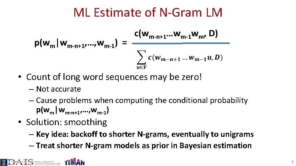
ML Estimate of N-Gram LM p(wm|wm-n+1, …, wm-1) = c(wm-n+1…wm-1 wm, D) • Count of long word sequences may be zero! – Not accurate – Cause problems when computing the conditional probability p(wm|wm-n+1, …, wm-1) • Solution: smoothing – Key idea: backoff to shorter N-grams, eventually to unigrams – Treat shorter N-gram models as prior in Bayesian estimation 8

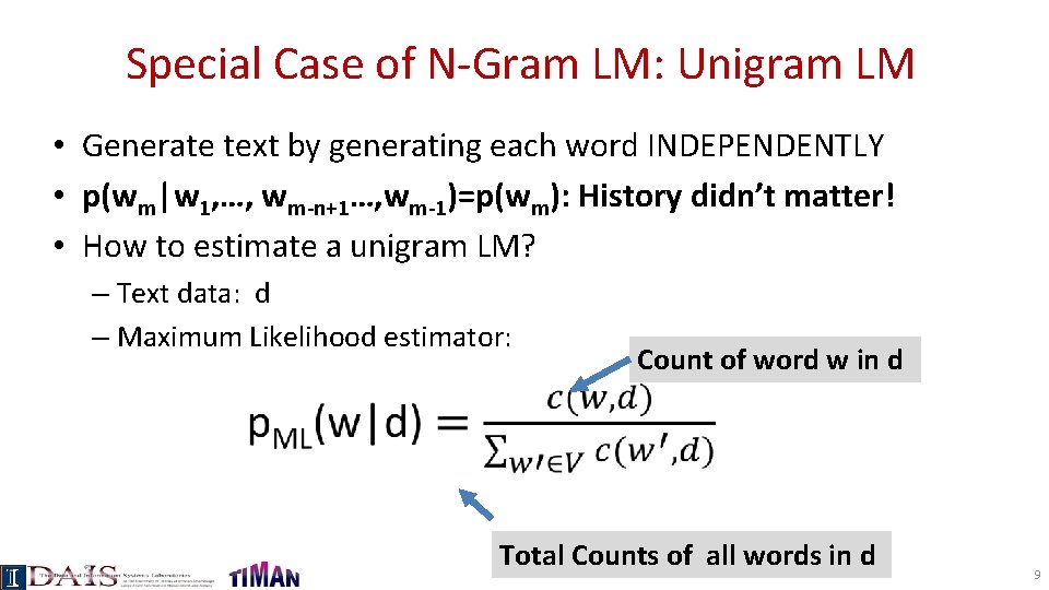
Special Case of N-Gram LM: Unigram LM • Generate text by generating each word INDEPENDENTLY • p(wm|w 1, …, wm-n+1…, wm-1)=p(wm): History didn’t matter! • How to estimate a unigram LM? – Text data: d – Maximum Likelihood estimator: Count of word w in d Total Counts of all words in d 9

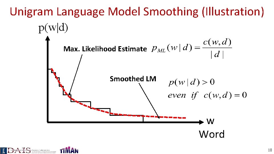
Unigram Language Model Smoothing (Illustration) p(w|d) Max. Likelihood Estimate Smoothed LM w Word 10

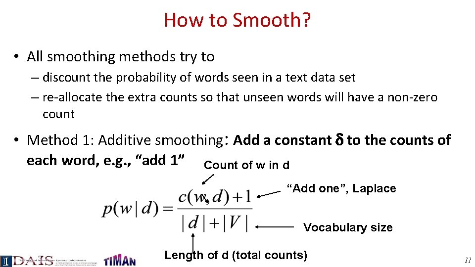
How to Smooth? • All smoothing methods try to – discount the probability of words seen in a text data set – re-allocate the extra counts so that unseen words will have a non-zero count • Method 1: Additive smoothing: Add a constant to the counts of each word, e. g. , “add 1” Count of w in d “Add one”, Laplace Vocabulary size Length of d (total counts) 11

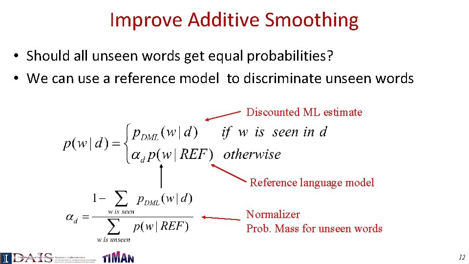
Improve Additive Smoothing • Should all unseen words get equal probabilities? • We can use a reference model to discriminate unseen words Discounted ML estimate Reference language model Normalizer Prob. Mass for unseen words 12

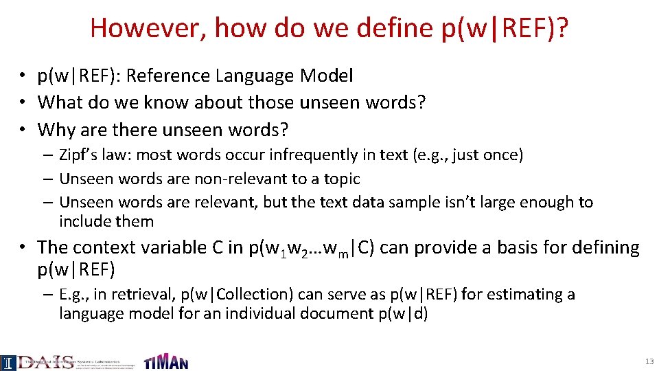
However, how do we define p(w|REF)? • p(w|REF): Reference Language Model • What do we know about those unseen words? • Why are there unseen words? – Zipf’s law: most words occur infrequently in text (e. g. , just once) – Unseen words are non-relevant to a topic – Unseen words are relevant, but the text data sample isn’t large enough to include them • The context variable C in p(w 1 w 2…wm|C) can provide a basis for defining p(w|REF) – E. g. , in retrieval, p(w|Collection) can serve as p(w|REF) for estimating a language model for an individual document p(w|d) 13

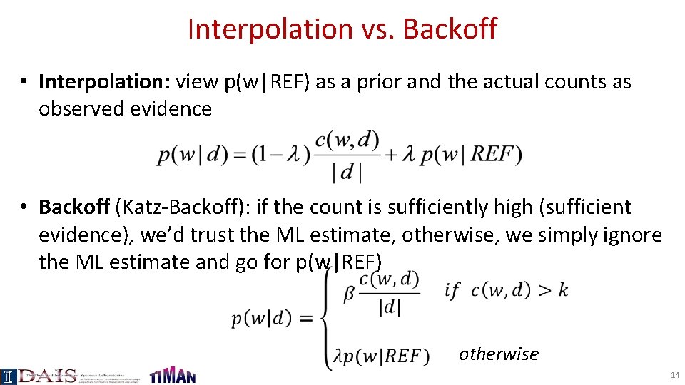
Interpolation vs. Backoff • Interpolation: view p(w|REF) as a prior and the actual counts as observed evidence • Backoff (Katz-Backoff): if the count is sufficiently high (sufficient evidence), we’d trust the ML estimate, otherwise, we simply ignore the ML estimate and go for p(w|REF) otherwise 14

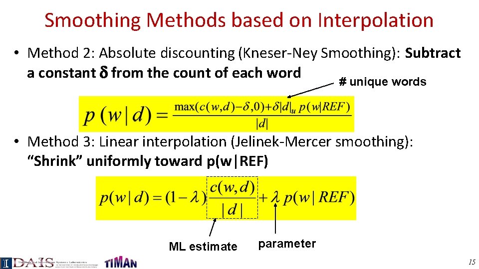
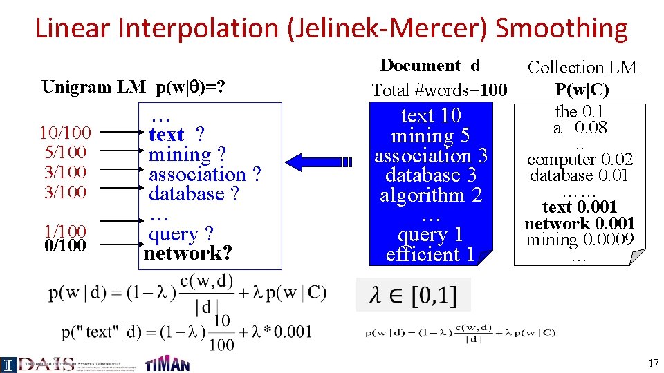
Smoothing Methods based on Interpolation • Method 2: Absolute discounting (Kneser-Ney Smoothing): Subtract a constant from the count of each word # unique words • Method 3: Linear interpolation (Jelinek-Mercer smoothing): “Shrink” uniformly toward p(w|REF) ML estimate parameter 15

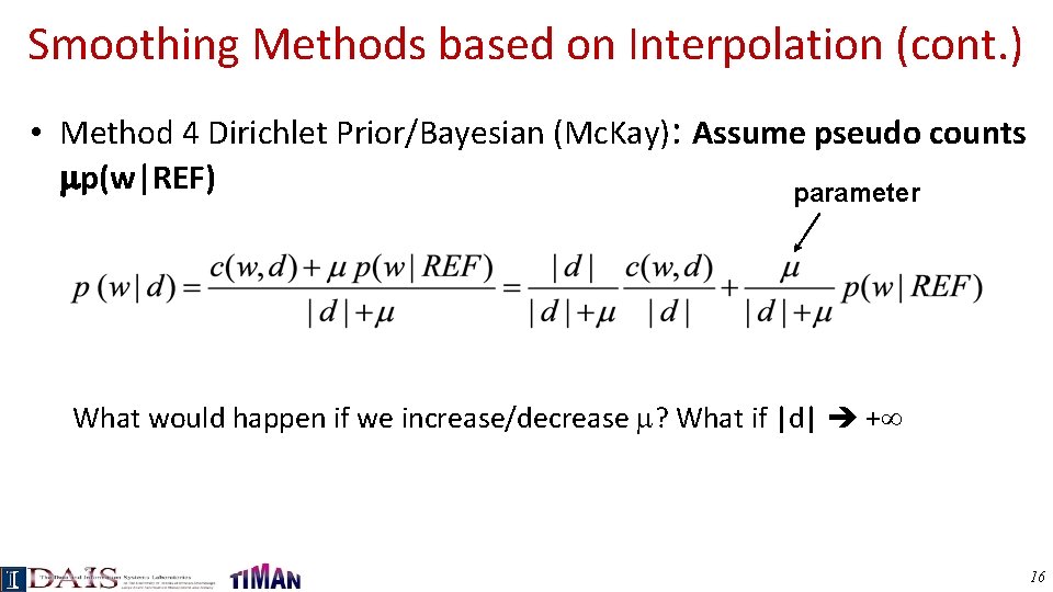
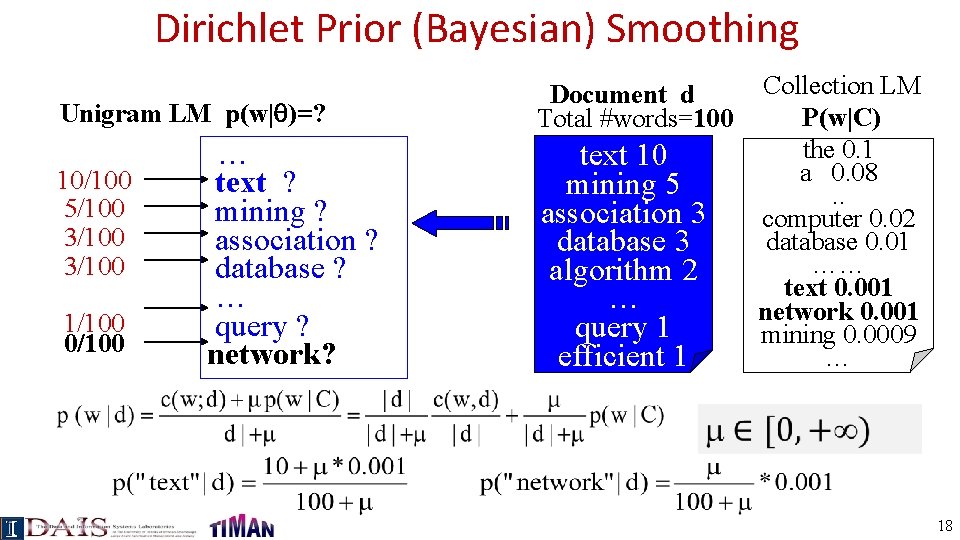
Smoothing Methods based on Interpolation (cont. ) • Method 4 Dirichlet Prior/Bayesian (Mc. Kay): Assume pseudo counts p(w|REF) parameter What would happen if we increase/decrease ? What if |d| + 16

Linear Interpolation (Jelinek-Mercer) Smoothing Unigram LM p(w| )=? 10/100 5/100 3/100 1/100 0/100 … text ? mining ? association ? database ? … query ? network? Document d Total #words=100 text 10 mining 5 association 3 database 3 algorithm 2 … query 1 efficient 1 Collection LM P(w|C) the 0. 1 a 0. 08. . computer 0. 02 database 0. 01 …… text 0. 001 network 0. 001 mining 0. 0009 … 17

Dirichlet Prior (Bayesian) Smoothing Unigram LM p(w| )=? 10/100 5/100 3/100 1/100 0/100 … text ? mining ? association ? database ? … query ? network? Document d Total #words=100 text 10 mining 5 association 3 database 3 algorithm 2 … query 1 efficient 1 Collection LM P(w|C) the 0. 1 a 0. 08. . computer 0. 02 database 0. 01 …… text 0. 001 network 0. 001 mining 0. 0009 … 18

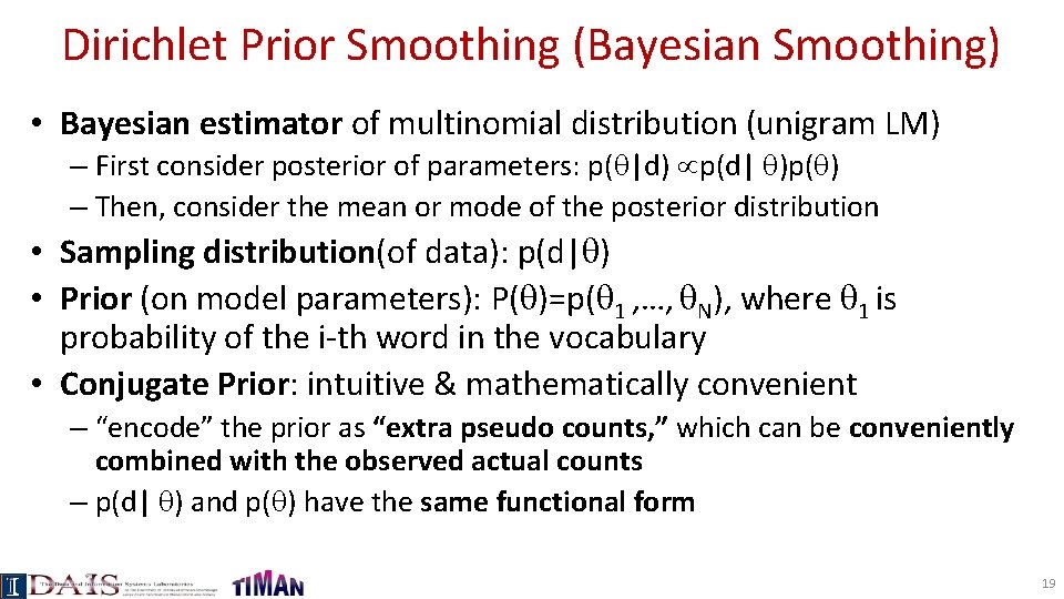
Dirichlet Prior Smoothing (Bayesian Smoothing) • Bayesian estimator of multinomial distribution (unigram LM) – First consider posterior of parameters: p( |d) p(d| )p( ) – Then, consider the mean or mode of the posterior distribution • Sampling distribution(of data): p(d| ) • Prior (on model parameters): P( )=p( 1 , …, N), where 1 is probability of the i-th word in the vocabulary • Conjugate Prior: intuitive & mathematically convenient – “encode” the prior as “extra pseudo counts, ” which can be conveniently combined with the observed actual counts – p(d| ) and p( ) have the same functional form 19

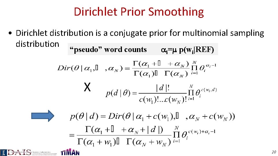
Dirichlet Prior Smoothing • Dirichlet distribution is a conjugate prior for multinomial sampling distribution “pseudo” word counts i= p(wi|REF) X 20

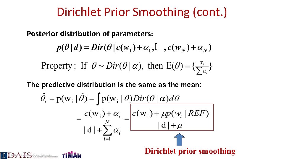
Dirichlet Prior Smoothing (cont. ) Posterior distribution of parameters: The predictive distribution is the same as the mean: Dirichlet prior smoothing

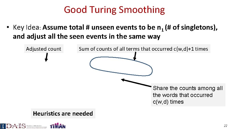
Good Turing Smoothing • Key Idea: Assume total # unseen events to be n 1 (# of singletons), and adjust all the seen events in the same way Adjusted count Sum of counts of all terms that occurred c(w, d)+1 times Share the counts among all the words that occurred c(w, d) times Heuristics are needed 22

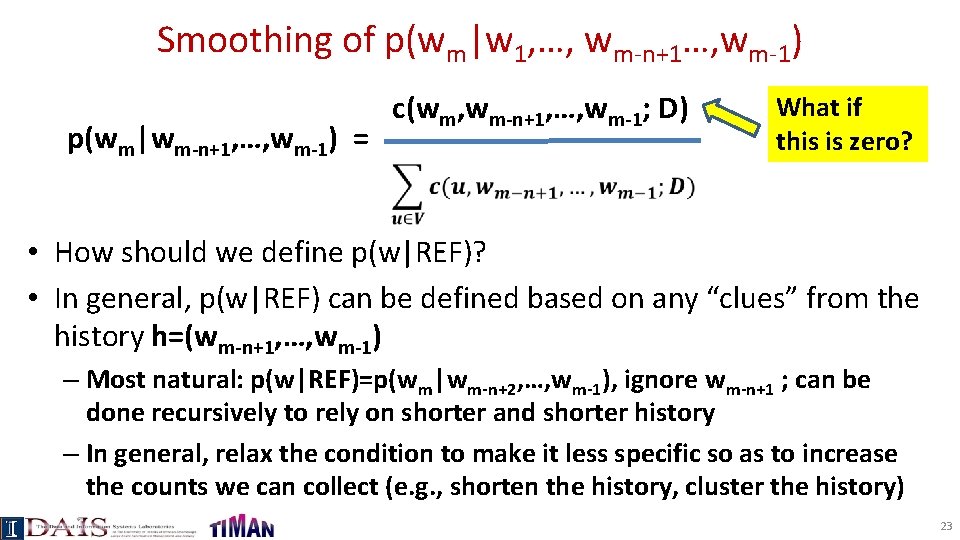
Smoothing of p(wm|w 1, …, wm-n+1…, wm-1) p(wm|wm-n+1, …, wm-1) = c(wm, wm-n+1, …, wm-1; D) What if this is zero? • How should we define p(w|REF)? • In general, p(w|REF) can be defined based on any “clues” from the history h=(wm-n+1, …, wm-1) – Most natural: p(w|REF)=p(wm|wm-n+2, …, wm-1), ignore wm-n+1 ; can be done recursively to rely on shorter and shorter history – In general, relax the condition to make it less specific so as to increase the counts we can collect (e. g. , shorten the history, cluster the history) 23

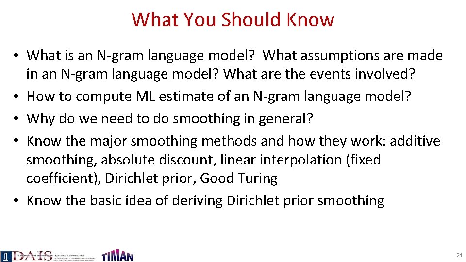
What You Should Know • What is an N-gram language model? What assumptions are made in an N-gram language model? What are the events involved? • How to compute ML estimate of an N-gram language model? • Why do we need to do smoothing in general? • Know the major smoothing methods and how they work: additive smoothing, absolute discount, linear interpolation (fixed coefficient), Dirichlet prior, Good Turing • Know the basic idea of deriving Dirichlet prior smoothing 24