New physical constraints for multiframe blind deconvolution Roberto

New physical constraints for multi-frame blind deconvolution Roberto Baena Gallé Real Academia de Artes y Ciencias de Barcelona Szymon Gładysz Fraunhofer Institute of Optronics, System Technologies and Image Exploitation Laurent Mugnier ONERA - The French Aerospace Lab Rao Gudimetla, Robert L. Johnson and Lee Kann Air Force Research Laboratory © Fraunhofer IOSB 1

Motivation and objectives No AO Motivation Speckle imaging and multi-frame blind deconvolution work well only for very short integration times and very narrow bandwidths. Adaptive optics (AO) at visible wavelengths is very hard. Attainment of diffraction-limited resolution is only possible in With AO conjunction with deconvolution. Objectives Develop a new theory of statistics of images blurred by With AO + deconv. turbulence. Test if inclusion of this theory in deconvolution removes the need for human intervention. © Fraunhofer IOSB 2

Bayesian framework i : dataset o : object h : PSF Likelihood when noise is Gaussian Prior on the PSFs P(h) can be formulated in: spatial domain (focal-plane intensity statistics). Fourier domain (statistics of the optical transfer function, OTF). © Fraunhofer IOSB 3

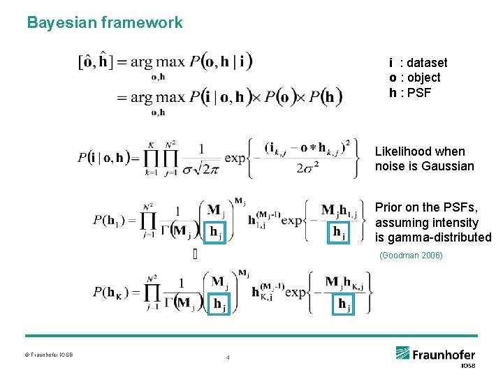
Bayesian framework i : dataset o : object h : PSF Likelihood when noise is Gaussian Prior on the PSFs, assuming intensity is gamma-distributed (Goodman 2006) © Fraunhofer IOSB 4

Estimation of r 0 ■ Fried’s parameter r 0 can be estimated directly from the data: (Spectral ratio. von der Lühe 1984) (Fourier contrast. Gladysz et al. 2012) © Fraunhofer IOSB 5

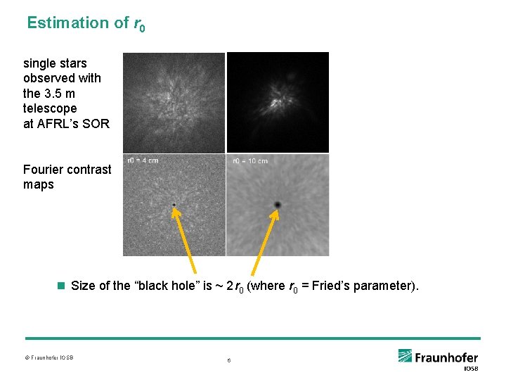
Estimation of r 0 single stars observed with the 3. 5 m telescope at AFRL’s SOR Fourier contrast maps Size of the “black hole” is ~ 2 r 0 (where r 0 = Fried’s parameter). © Fraunhofer IOSB 6

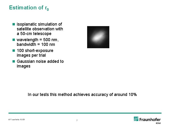
Estimation of r 0 isoplanatic simulation of satellite observation with a 50 -cm telescope wavelength = 500 nm, bandwidth = 100 nm 100 short-exposure images per trial Gaussian noise added to images In our tests this method achieves accuracy of around 10% © Fraunhofer IOSB 7

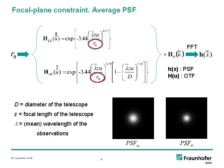
Focal-plane constraint. Average PSF FFT h(x) : PSF H(u) : OTF D = diameter of the telescope z = focal length of the telescope = (mean) wavelength of the observations © Fraunhofer IOSB 8

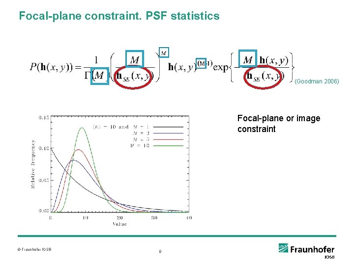
Focal-plane constraint. PSF statistics (Goodman 2006) Focal-plane or image constraint © Fraunhofer IOSB 9

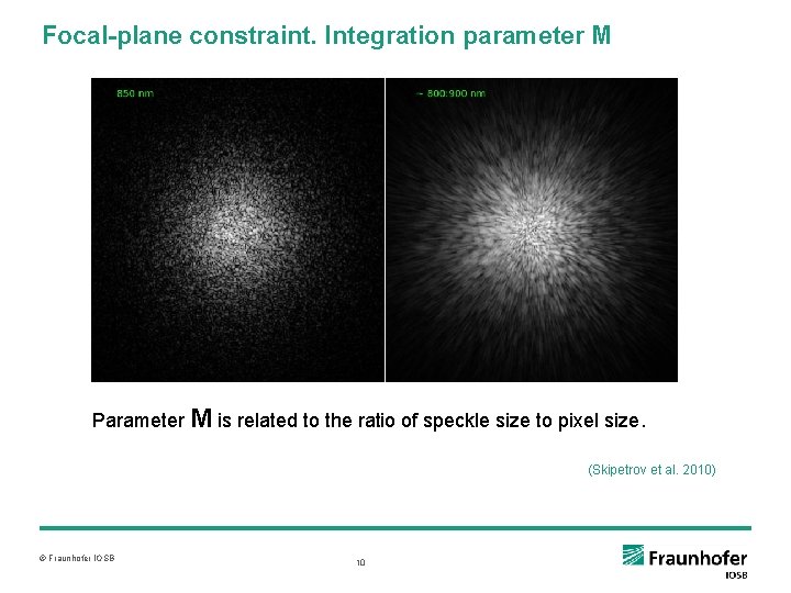
Focal-plane constraint. Integration parameter M Parameter M is related to the ratio of speckle size to pixel size. (Skipetrov et al. 2010) © Fraunhofer IOSB 10

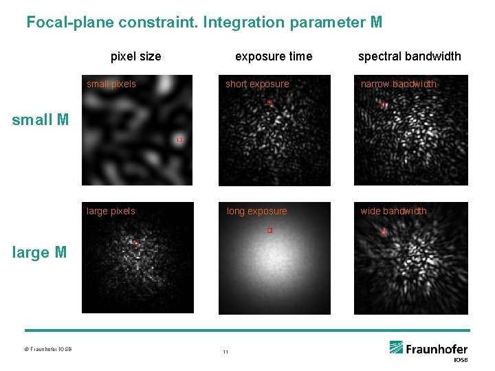
Focal-plane constraint. Integration parameter M pixel size small pixels exposure time short exposure spectral bandwidth narrow bandwidth small M large pixels long exposure large M © Fraunhofer IOSB 11 wide bandwidth

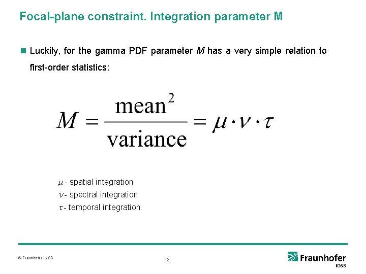
Focal-plane constraint. Integration parameter M Luckily, for the gamma PDF parameter M has a very simple relation to first-order statistics: - spatial integration - spectral integration - temporal integration © Fraunhofer IOSB 12

Focal-plane constraint in the Fourier domain For large D/r 0 real and imaginary parts of the OTF are Gaussian random variables. Models are needed for means and variances of real and imaginary parts of the OTF. © Fraunhofer IOSB 13

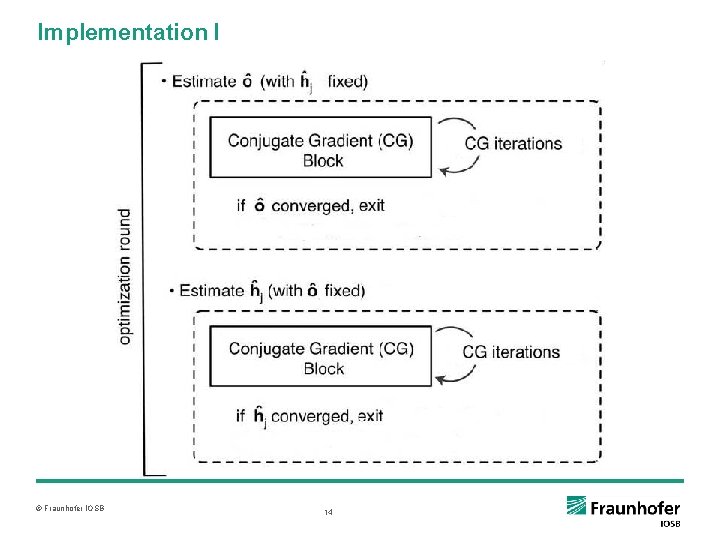
Implementation I © Fraunhofer IOSB 14

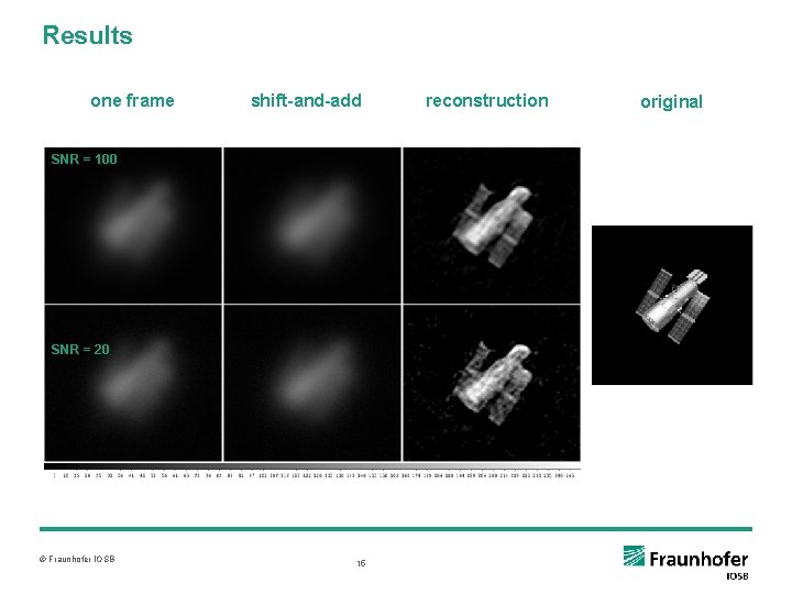
Results one frame shift-and-add SNR = 100 SNR = 20 © Fraunhofer IOSB 15 reconstruction original

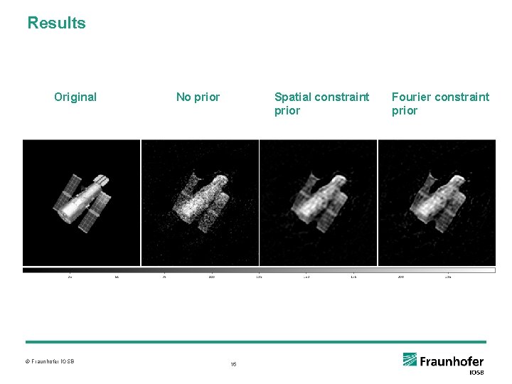
Results Original © Fraunhofer IOSB Spatial constraint prior No prior 16 Fourier constraint prior

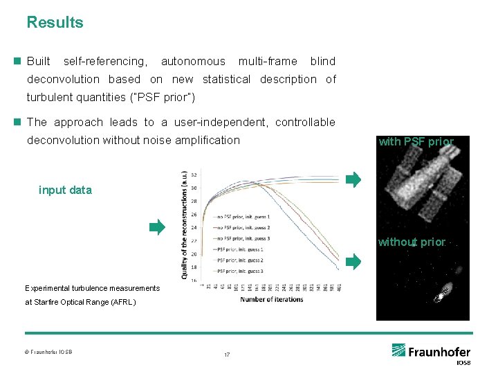
Results Built self-referencing, autonomous multi-frame blind deconvolution based on new statistical description of turbulent quantities (“PSF prior”) The approach leads to a user-independent, controllable deconvolution without noise amplification with PSF prior input data without prior Experimental turbulence measurements at Starfire Optical Range (AFRL) © Fraunhofer IOSB 17

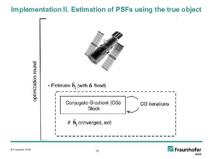
Implementation II. Estimation of PSFs using the true object © Fraunhofer IOSB 18

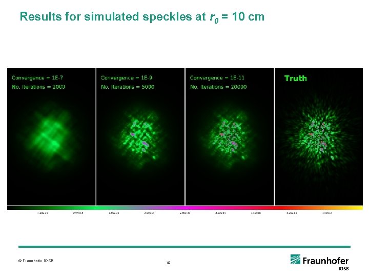
Results for simulated speckles at r 0 = 10 cm © Fraunhofer IOSB 19

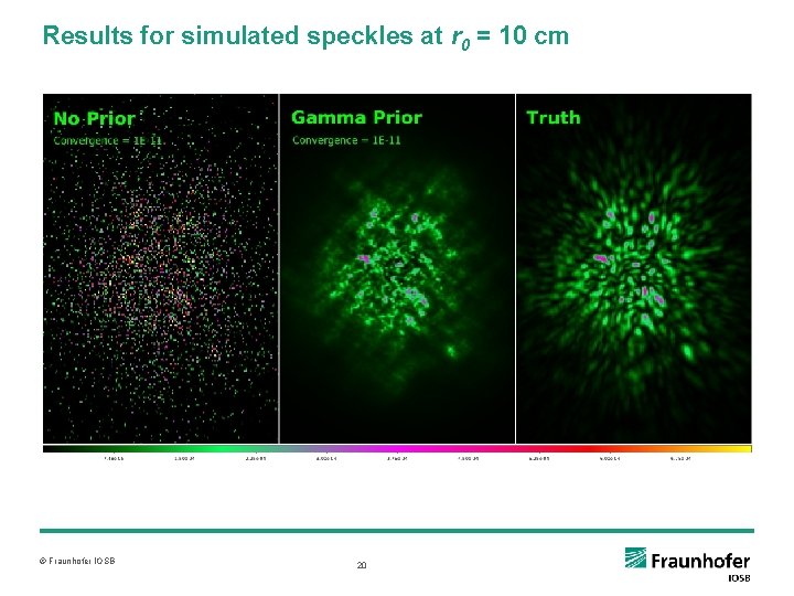
Results for simulated speckles at r 0 = 10 cm © Fraunhofer IOSB 20

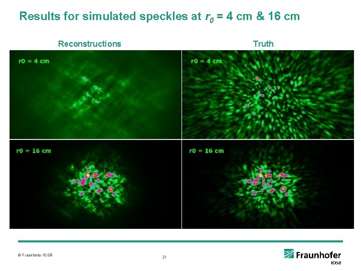
Results for simulated speckles at r 0 = 4 cm & 16 cm Reconstructions

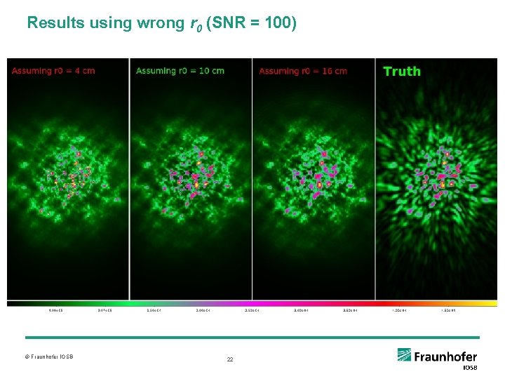
Results using wrong r 0 (SNR = 100) © Fraunhofer IOSB 22

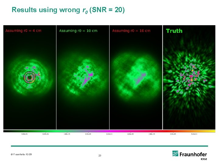
Results using wrong r 0 (SNR = 20) © Fraunhofer IOSB 23

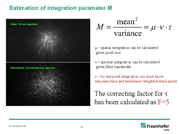
Estimation of integration parameter M μ – spatial integration can be calculated given pixel size ν – spectral integration can be calculated given filter bandwidth τ – for temporal integration one must know exposure time and turbulence-weighted wind speed The correcting factor for τ has been calculated as F=5 © Fraunhofer IOSB 24

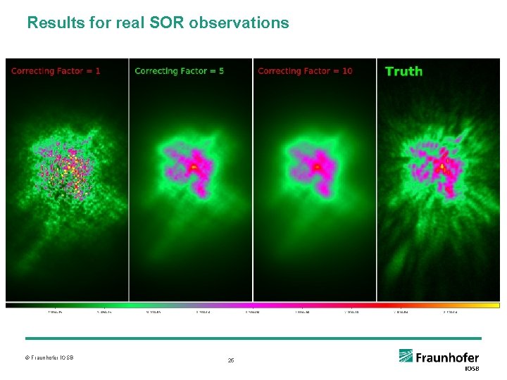
Results for real SOR observations © Fraunhofer IOSB 25

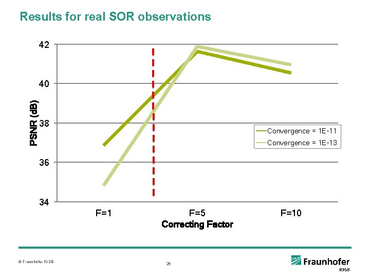
Results for real SOR observations 42 PSNR (d. B) 40 38 Convergence = 1 E-11 Convergence = 1 E-13 36 34 F=1 © Fraunhofer IOSB F=5 Correcting Factor 26 F=10

Summary We are developing a new framework for deconvolution of images of space-based objects for the Air Force Research Lab. The algorithms must be autonomous. Average PSF is derived directly from the data. No hyperparameters are needed. Priors on the PSFs are derived from physics of the imaging process. Spatial-, and Fourier-frequency-based priors delay the onset of noise amplification. Objects and PSFs are reconstructed correctly. © Fraunhofer IOSB 27

New physical constraints for multi-frame blind deconvolution Effort sponsored by U. S. Air Force Office of Scientific Research, Air Force Materiel Command, under grant FA 8655 -12 -1 -2115. © Fraunhofer IOSB 28