Neurophysics Part 1 Neural encoding and decoding Ch

Neurophysics • Part 1: Neural encoding and decoding (Ch 1 -4) • Stimulus to response (1 -2) • Response to stimulus, information in spikes (3 -4) • Part 2: Neurons and Neural circuits (Ch 5 -7) • Classical neuron model (5) • Extensions (6) • Neural networks (7) • Part 3: Adaptation and learning (Ch 8 -10) • Synaptic plasticity (8) • Classical conditioning and RL (9) • Pattern recognition and machine learning methods (10)

Chapter 1

Outline • • Neurons Firing rate Tuning curves Deviation from the mean: statistical description – Spike triggered average – Point process, Poisson process • Poisson process – Homogeneous, Inhomogeneous – Experimental validation – shortcomings

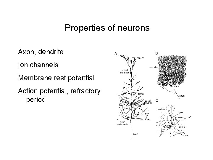
Properties of neurons Axon, dendrite Ion channels Membrane rest potential Action potential, refractory period

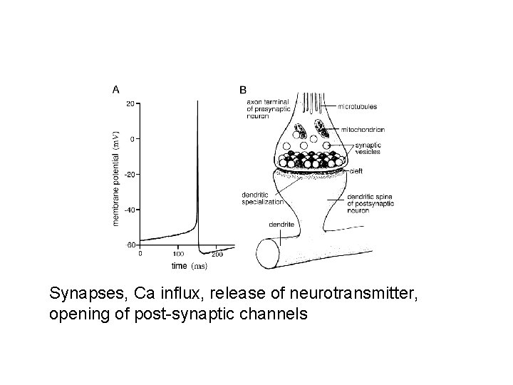
Synapses, Ca influx, release of neurotransmitter, opening of post-synaptic channels

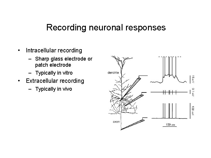
Recording neuronal responses • Intracellular recording – Sharp glass electrode or patch electrode – Typically in vitro • Extracellular recording – Typically in vivo

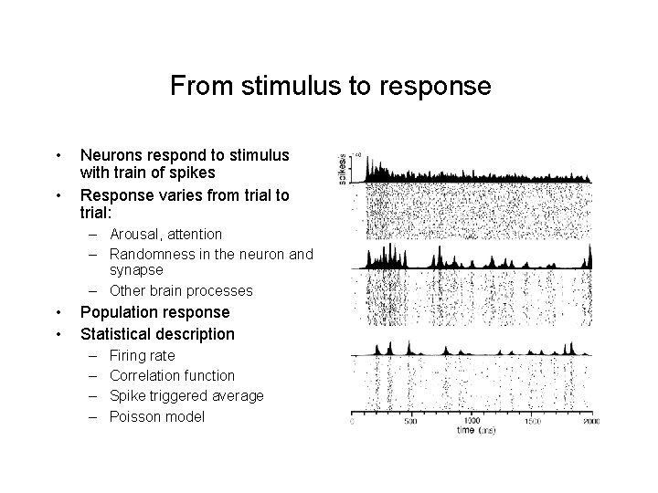
From stimulus to response • • Neurons respond to stimulus with train of spikes Response varies from trial to trial: – Arousal, attention – Randomness in the neuron and synapse – Other brain processes • • Population response Statistical description – – Firing rate Correlation function Spike triggered average Poisson model

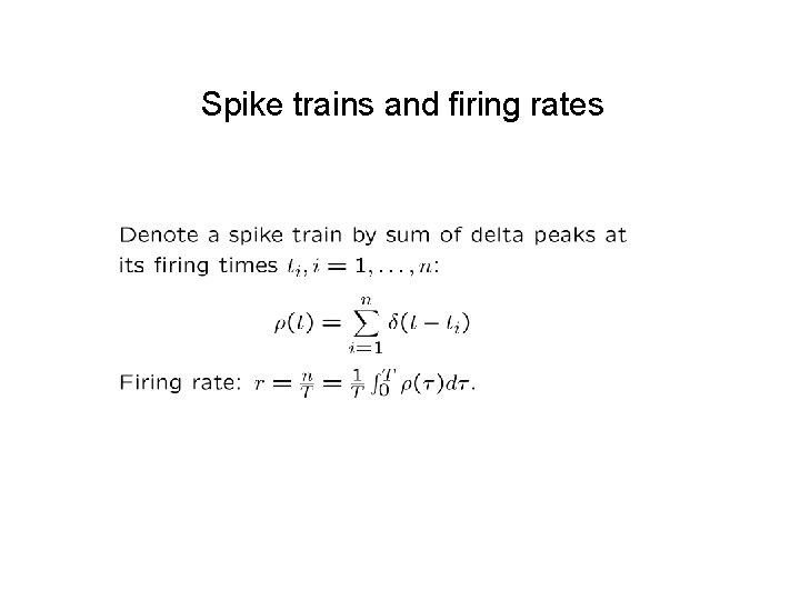
Spike trains and firing rates

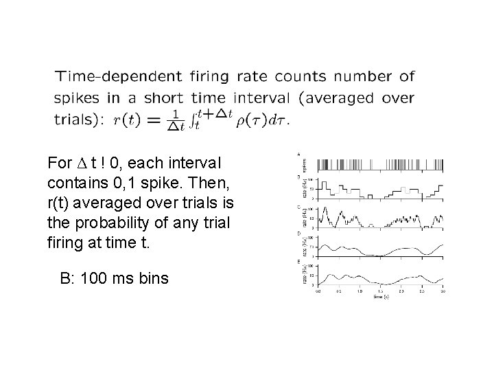
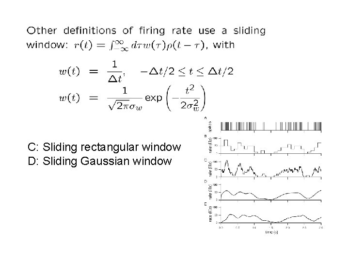
For Δ t ! 0, each interval contains 0, 1 spike. Then, r(t) averaged over trials is the probability of any trial firing at time t. B: 100 ms bins

C: Sliding rectangular window D: Sliding Gaussian window

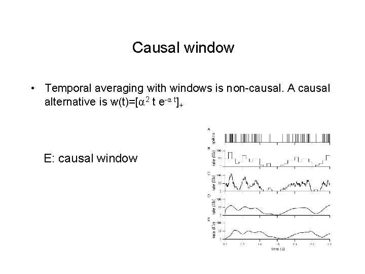
Causal window • Temporal averaging with windows is non-causal. A causal alternative is w(t)=[α 2 t e-α t]+ E: causal window

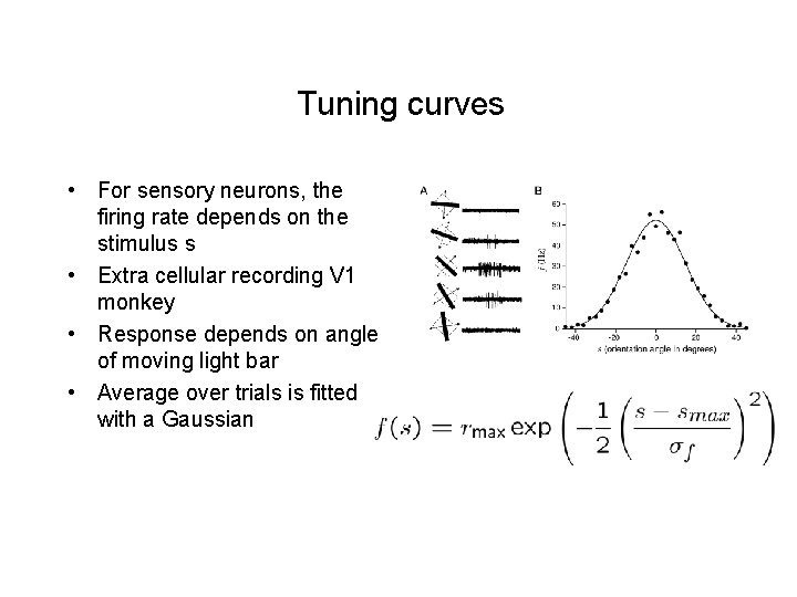
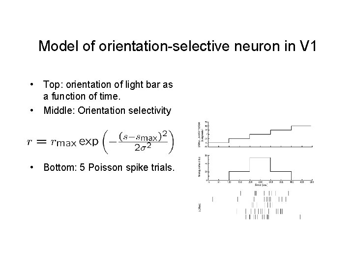
Tuning curves • For sensory neurons, the firing rate depends on the stimulus s • Extra cellular recording V 1 monkey • Response depends on angle of moving light bar • Average over trials is fitted with a Gaussian

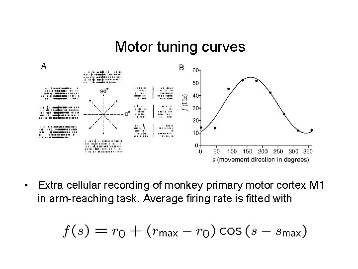
Motor tuning curves • Extra cellular recording of monkey primary motor cortex M 1 in arm-reaching task. Average firing rate is fitted with

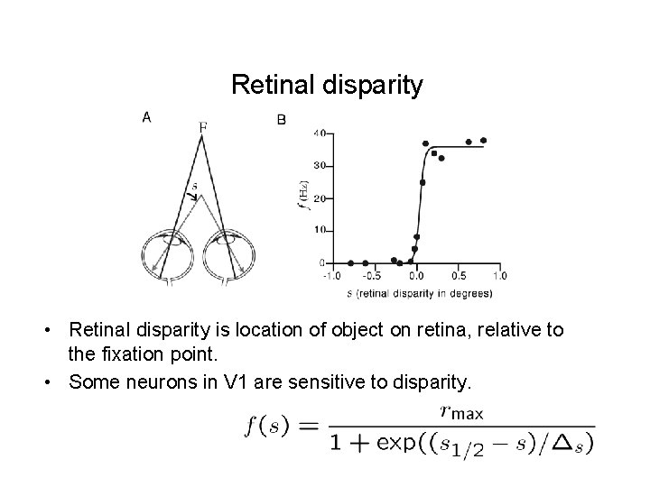
Retinal disparity • Retinal disparity is location of object on retina, relative to the fixation point. • Some neurons in V 1 are sensitive to disparity.

Spike-count variability • Tuning curves model average behavior. • Deviations of individual trials are given by a noise model. – Additive noise is independent of stimulus r=f(s)+ξ – Multiplicative noise is proportional to stimulus r=f(s) ξ • statistical description – Spike triggered average – Correlations

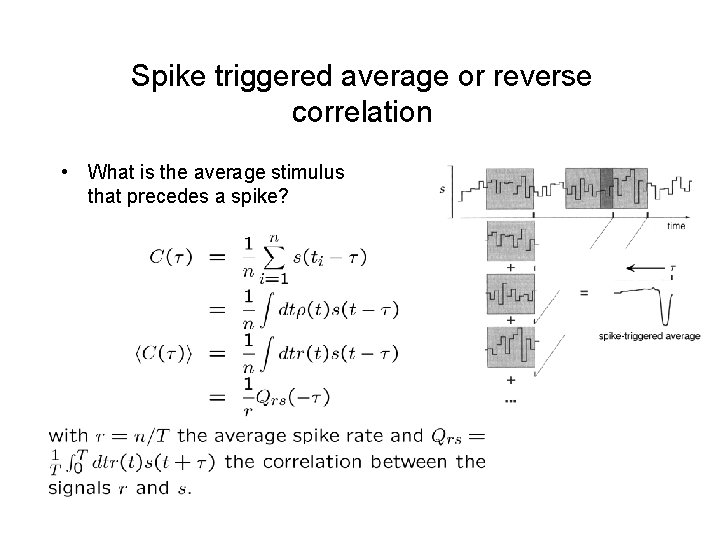
Spike triggered average or reverse correlation • What is the average stimulus that precedes a spike?

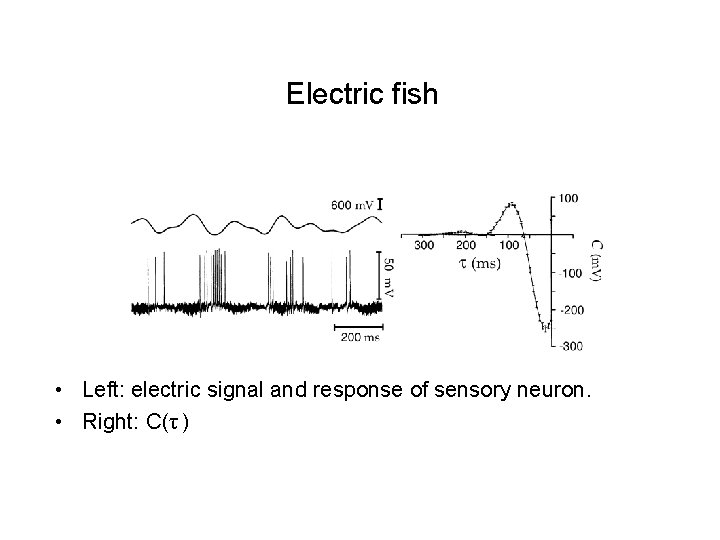
Electric fish • Left: electric signal and response of sensory neuron. • Right: C(τ )

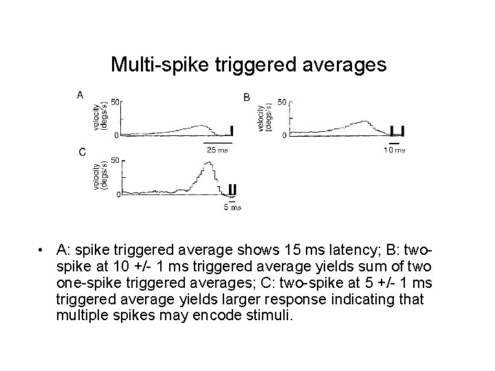
Multi-spike triggered averages • A: spike triggered average shows 15 ms latency; B: twospike at 10 +/- 1 ms triggered average yields sum of two one-spike triggered averages; C: two-spike at 5 +/- 1 ms triggered average yields larger response indicating that multiple spikes may encode stimuli.

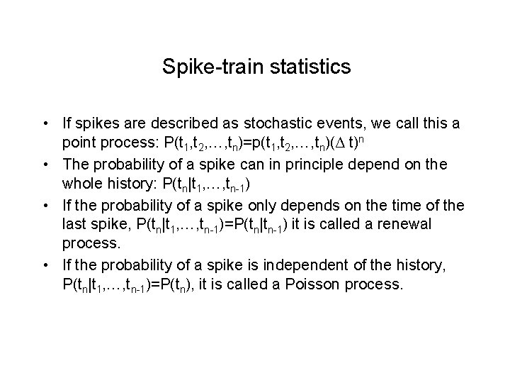
Spike-train statistics • If spikes are described as stochastic events, we call this a point process: P(t 1, t 2, …, tn)=p(t 1, t 2, …, tn)(Δ t)n • The probability of a spike can in principle depend on the whole history: P(tn|t 1, …, tn-1) • If the probability of a spike only depends on the time of the last spike, P(tn|t 1, …, tn-1)=P(tn|tn-1) it is called a renewal process. • If the probability of a spike is independent of the history, P(tn|t 1, …, tn-1)=P(tn), it is called a Poisson process.

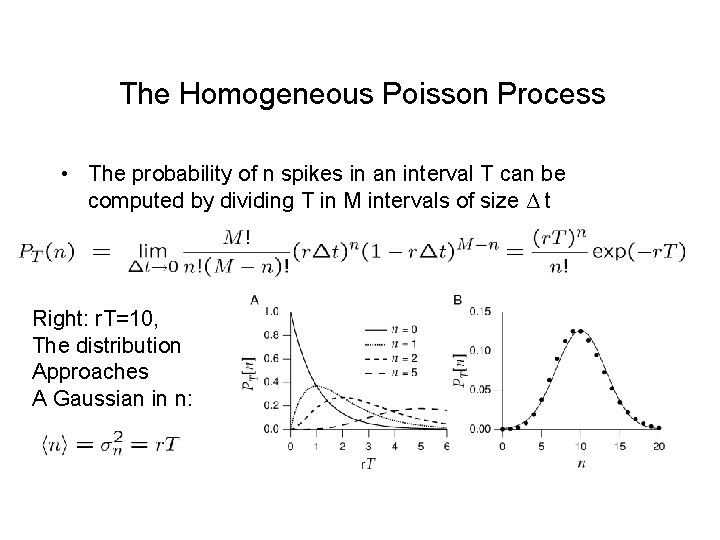
The Homogeneous Poisson Process • The probability of n spikes in an interval T can be computed by dividing T in M intervals of size Δ t Right: r. T=10, The distribution Approaches A Gaussian in n:

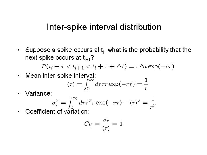
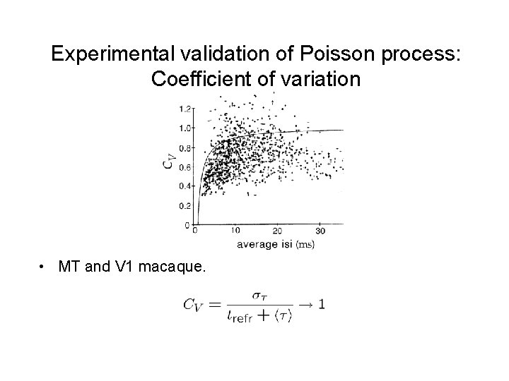
Inter-spike interval distribution • Suppose a spike occurs at t. I, what is the probability that the next spike occurs at t. I+1? • Mean inter-spike interval: • Variance: • Coefficient of variation:

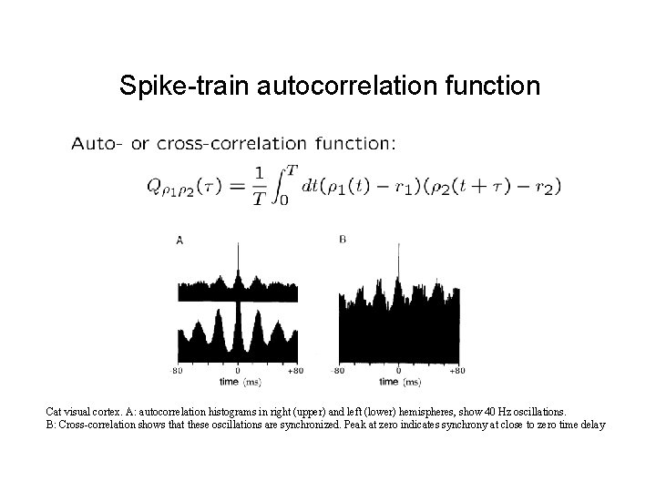
Spike-train autocorrelation function Cat visual cortex. A: autocorrelation histograms in right (upper) and left (lower) hemispheres, show 40 Hz oscillations. B: Cross-correlation shows that these oscillations are synchronized. Peak at zero indicates synchrony at close to zero time delay

Autocorrelation for Poisson process

Inhomogeneous Poisson Process • Divide the interval [ti, ti+1] in M segments of length Δ t. • The probability of no spikes in [ti, ti+1] is

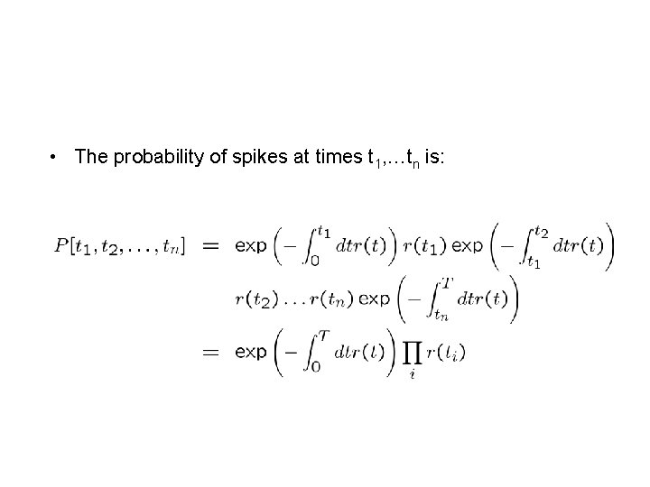
• The probability of spikes at times t 1, …tn is:

Poisson spike generation • Either – Choose small bins Δ t and generate with probability r(t)Δ t, or – Choose ti+1 -t. I from p(τ )=r exp(-r τ ) • Second method is much faster, but works for homogeneous Poisson processes only • It is further discussed in an exercise.

Model of orientation-selective neuron in V 1 • Top: orientation of light bar as a function of time. • Middle: Orientation selectivity • Bottom: 5 Poisson spike trials.

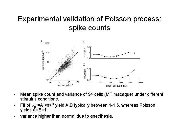
Experimental validation of Poisson process: spike counts • • • Mean spike count and variance of 94 cells (MT macaque) under different stimulus conditions. Fit of σ n 2=A <n>B yield A, B typically between 1 -1. 5, whereas Poisson yields A=B=1. variance higher than normal due to anesthesia.

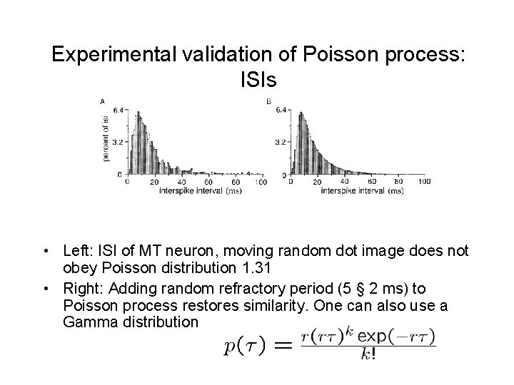
Experimental validation of Poisson process: ISIs • Left: ISI of MT neuron, moving random dot image does not obey Poisson distribution 1. 31 • Right: Adding random refractory period (5 § 2 ms) to Poisson process restores similarity. One can also use a Gamma distribution

Experimental validation of Poisson process: Coefficient of variation • MT and V 1 macaque.

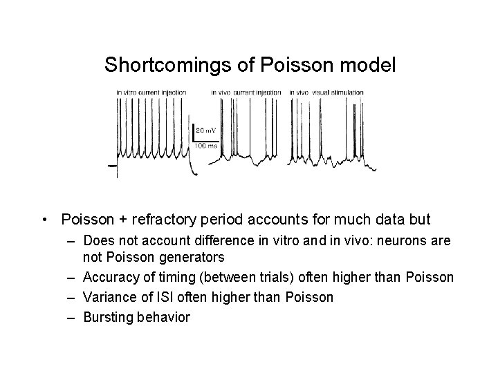
Shortcomings of Poisson model • Poisson + refractory period accounts for much data but – Does not account difference in vitro and in vivo: neurons are not Poisson generators – Accuracy of timing (between trials) often higher than Poisson – Variance of ISI often higher than Poisson – Bursting behavior

Types of coding: single neuron description • Independent-spike code: all information is in the rate r(t). This is a Poisson process • Correlation code: spike timing is history dependent. For instance a renewal process p(ti+1|ti) • Deviation from Poisson process typically less than 10 %.

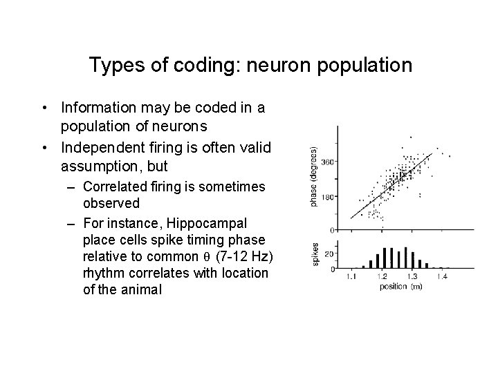
Types of coding: neuron population • Information may be coded in a population of neurons • Independent firing is often valid assumption, but – Correlated firing is sometimes observed – For instance, Hippocampal place cells spike timing phase relative to common θ (7 -12 Hz) rhythm correlates with location of the animal

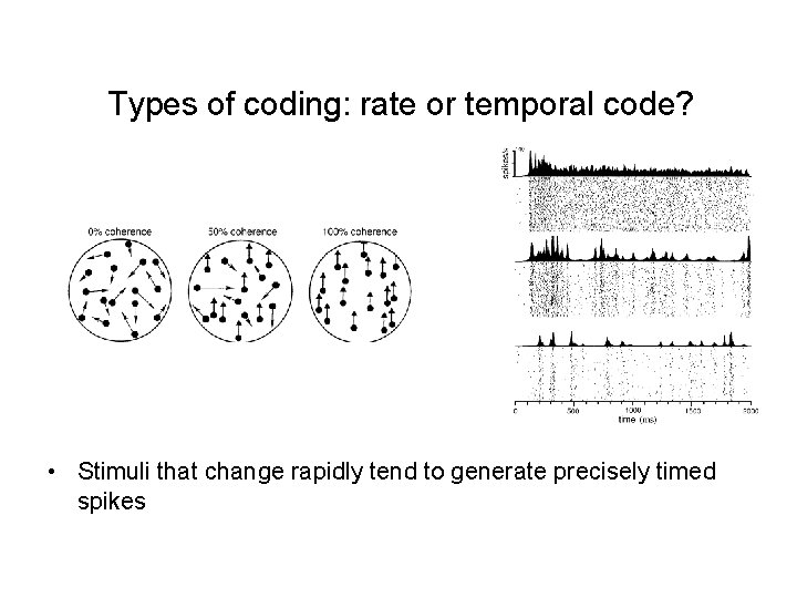
Types of coding: rate or temporal code? • Stimuli that change rapidly tend to generate precisely timed spikes

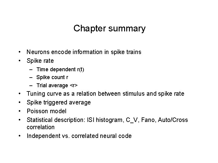
Chapter summary • Neurons encode information in spike trains • Spike rate – Time dependent r(t) – Spike count r – Trial average <r> • • Tuning curve as a relation between stimulus and spike rate Spike triggered average Poisson model Statistical description: ISI histogram, C_V, Fano, Auto/Cross correlation • Independent vs. correlated neural code

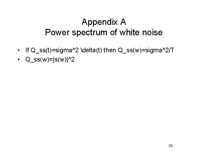
Appendix A Power spectrum of white noise • If Q_ss(t)=sigma^2 delta(t) then Q_ss(w)=sigma^2/T • Q_ss(w)=|s(w)|^2 36