Neural Networks Multistage regressionclassification model output function PPR

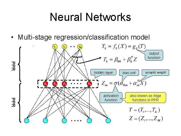
Neural Networks • Multi-stage regression/classification model output function PPR hidden layer PPR activation function bias unit synaptic weight also known as ridge functions in PPR

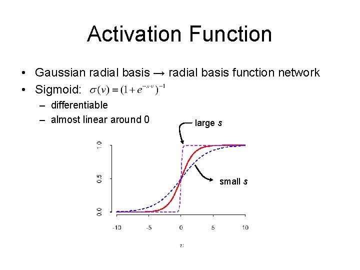
Activation Function • Gaussian radial basis → radial basis function network • Sigmoid: – differentiable – almost linear around 0 large s small s

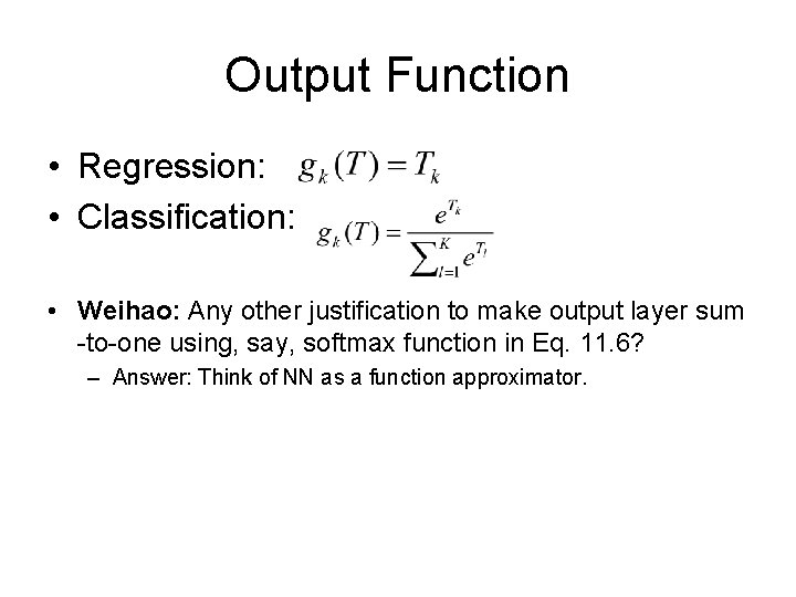
Output Function • Regression: • Classification: • Weihao: Any other justification to make output layer sum -to-one using, say, softmax function in Eq. 11. 6? – Answer: Think of NN as a function approximator.

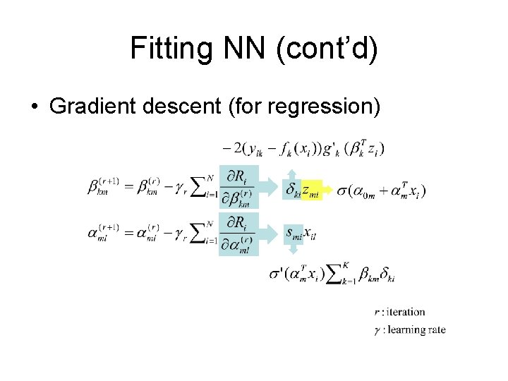
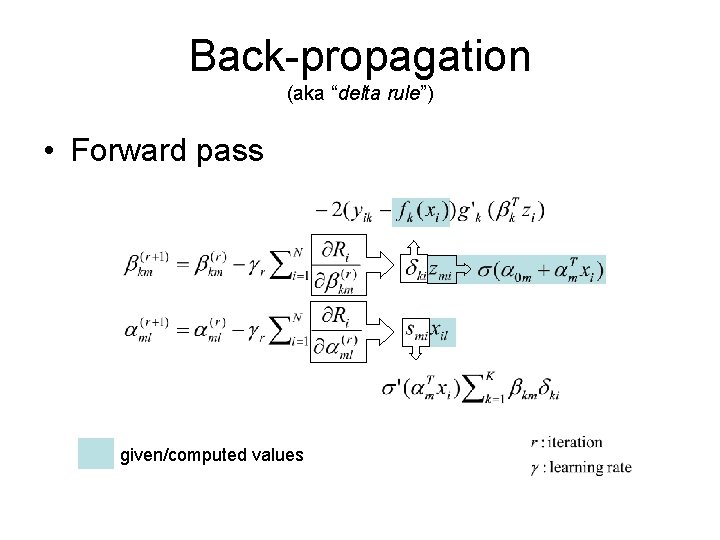
Fitting NN (cont’d) • Gradient descent (for regression)

Back-propagation (aka “delta rule”) • Forward pass given/computed values

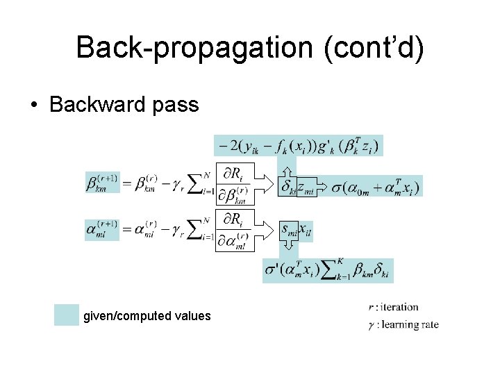
Back-propagation (cont’d) • Backward pass given/computed values

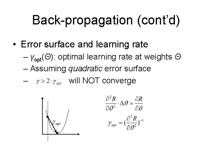
Back-propagation (cont’d) • Error surface and learning rate – γopt(Θ): optimal learning rate at weights Θ – Assuming quadratic error surface – will NOT converge

Back-propagation (cont’d) • Batch learning vs. online learning • Often too slow – Newton method not attractive (2 nd derivative too costly) – Use conjugate gradients, variable metric methods, etc. (Ch. 10, Numerical Recipes in C: http: //www. library. cornell. edu/nr/bookcpdf. html)

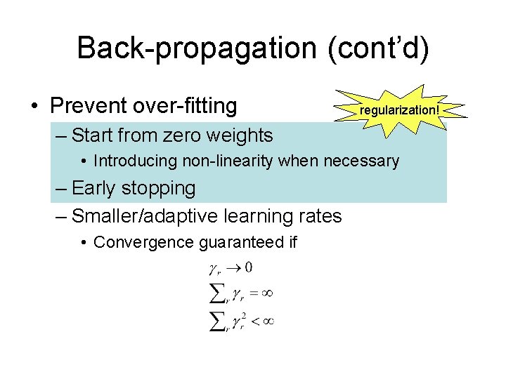
Back-propagation (cont’d) • Prevent over-fitting regularization! – Start from zero weights • Introducing non-linearity when necessary – Early stopping – Smaller/adaptive learning rates • Convergence guaranteed if

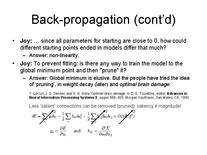
Back-propagation (cont’d) • Joy: … since all parameters for starting are close to 0, how could different starting points ended in models differ that much? – Answer: non-linearity. • Joy: To prevent fitting: is there any way to train the model to the global minimum point and then "prune" it? – Answer: Global minimum is elusive. But the people have tried the idea of ‘pruning’, in weight decay (later) and optimal brain damage: Y. Le. Cun, J. S. Denker, and S. A. Solla. Optimal brain damage. In D. S. Touretzky, editor, Advances in Neural Information Processing Systems II, pages 598 --605. Morgan Kaufmann, San Mateo, CA, 1990. Less ‘salient’ connections can be removed (pruned); saliency ≠ magnitude! 0 0 0

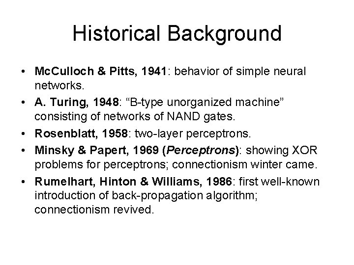
Historical Background • Mc. Culloch & Pitts, 1941: behavior of simple neural networks. • A. Turing, 1948: “B-type unorganized machine” consisting of networks of NAND gates. • Rosenblatt, 1958: two-layer perceptrons. • Minsky & Papert, 1969 (Perceptrons): showing XOR problems for perceptrons; connectionism winter came. • Rumelhart, Hinton & Williams, 1986: first well-known introduction of back-propagation algorithm; connectionism revived.

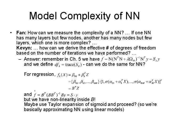
Model Complexity of NN • Fan: How can we measure the complexity of a NN? … If one NN has many layers but few nodes, another has many nodes but few layers, which one is more complex? … Kevyn: … how can we derive the effective # of degrees of freedom based on the number of iterations we have performed? … – Answer: remember in Ch. 5 we have and we define - can we do the same for NN? For regression, and but we have non-linearity inside B! Maybe use Taylor expansion of sigmoid and proceed? (so we’re basically approximating NN using linear models)

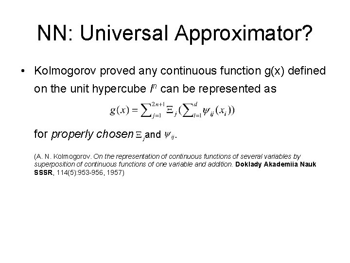
NN: Universal Approximator? • Kolmogorov proved any continuous function g(x) defined on the unit hypercube In can be represented as for properly chosen and . (A. N. Kolmogorov. On the representation of continuous functions of several variables by superposition of continuous functions of one variable and addition. Doklady Akademiia Nauk SSSR, 114(5): 953 -956, 1957)

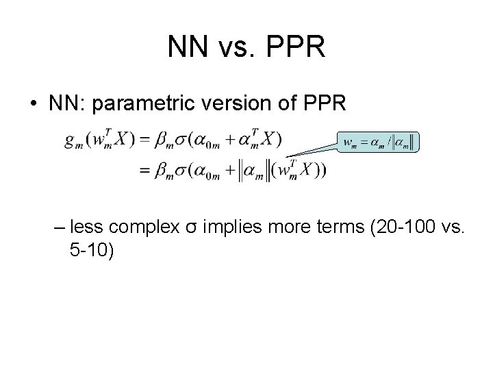
NN vs. PPR • NN: parametric version of PPR – less complex σ implies more terms (20 -100 vs. 5 -10)