Neural Network Approximation of Highdimensional Functions Peter Andras

Neural Network Approximation of Highdimensional Functions Peter Andras School of Computing and Mathematics Keele University p. andras@keele. ac. uk

Overview • High-dimensional functions and lowdimensional manifolds • Manifold mapping • Function approximation over low-dimensional projections • Performance evaluation • Conclusions 2

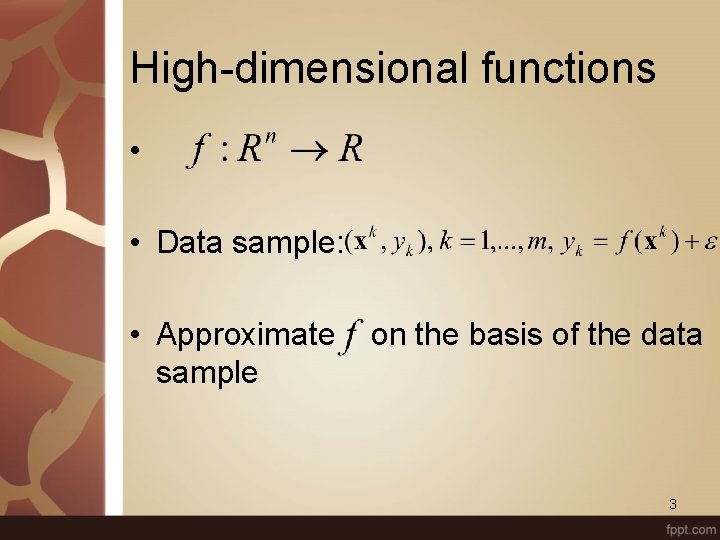
High-dimensional functions • • Data sample: • Approximate sample on the basis of the data 3

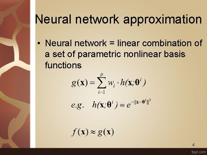
Neural network approximation • Neural network = linear combination of a set of parametric nonlinear basis functions 4

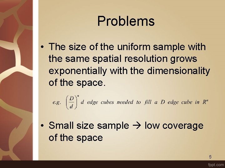
Problems • The size of the uniform sample with the same spatial resolution grows exponentially with the dimensionality of the space. • Small size sample low coverage of the space 5

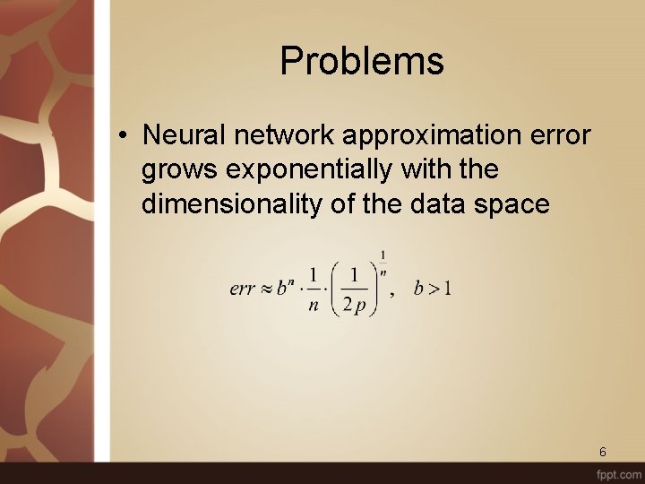
Problems • Neural network approximation error grows exponentially with the dimensionality of the data space 6

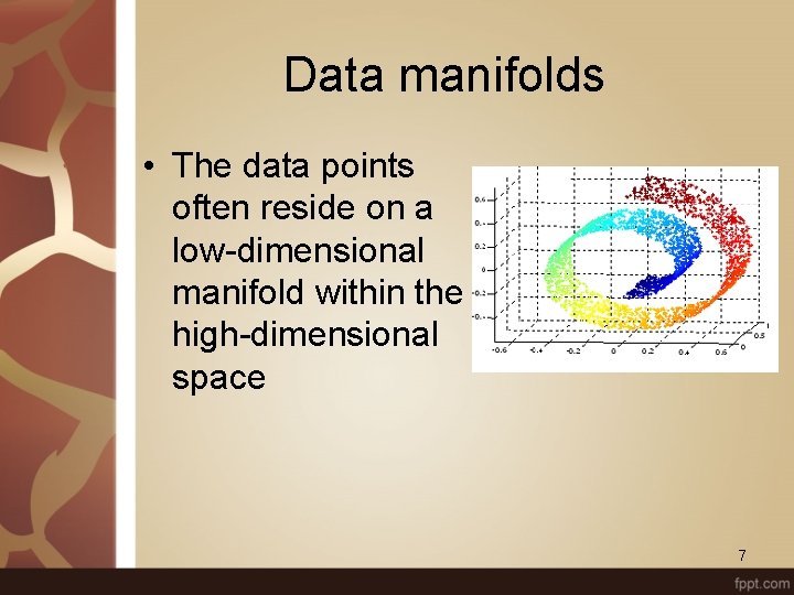
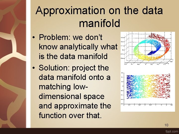
Data manifolds • The data points often reside on a low-dimensional manifold within the high-dimensional space 7

Data manifolds • Reasons: – Interdependent components of the measured data vectors – Much less degrees of freedoms in the behaviour of the underlying system than the number of simultaneous measurements – Nonlinear default geometry of the measured system 8

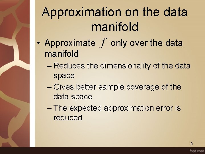
Approximation on the data manifold • Approximate manifold only over the data – Reduces the dimensionality of the data space – Gives better sample coverage of the data space – The expected approximation error is reduced 9

Approximation on the data manifold • Problem: we don’t know analytically what is the data manifold • Solution: project the data manifold onto a matching lowdimensional space and approximate the function over that. 10

Manifold mapping • Dimensionality estimation – Local principal component analysis • Low-dimensional mapping with preservation of topological organisation of the manifold: – Self-organising maps – Local linear embedding – Both: unsupervised learning 11

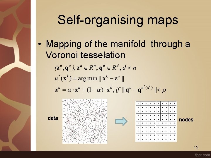
Self-organising maps • Mapping of the manifold through a Voronoi tesselation data nodes 12

Self-organising maps • SOM: learns the data distribution over the manifold and projects the learned Voronoi tesselation onto the low-dimensional space • The neighbourhood structure (topology) of the manifold is preserved 13

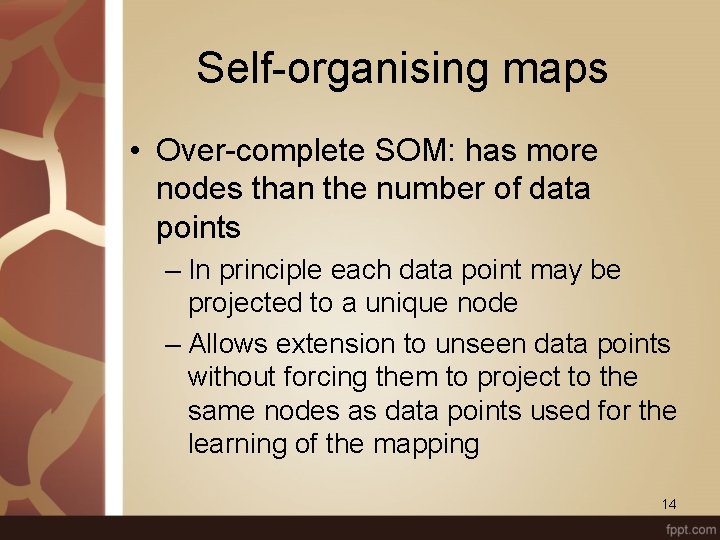
Self-organising maps • Over-complete SOM: has more nodes than the number of data points – In principle each data point may be projected to a unique node – Allows extension to unseen data points without forcing them to project to the same nodes as data points used for the learning of the mapping 14

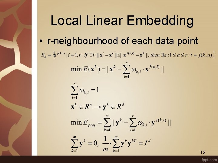
Local Linear Embedding • r-neighbourhood of each data point 15

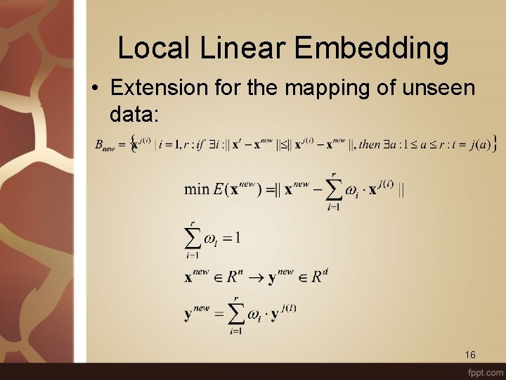
Local Linear Embedding • Extension for the mapping of unseen data: 16

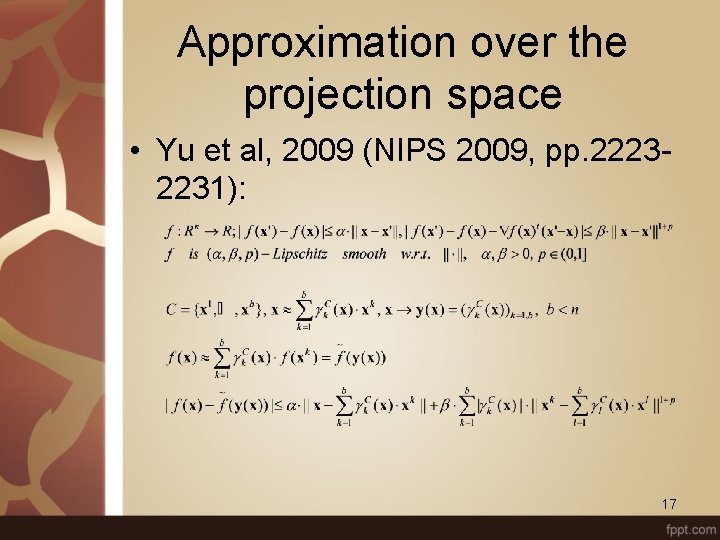
Approximation over the projection space • Yu et al, 2009 (NIPS 2009, pp. 22232231): 17

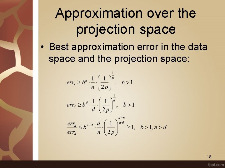
Approximation over the projection space • Best approximation error in the data space and the projection space: 18

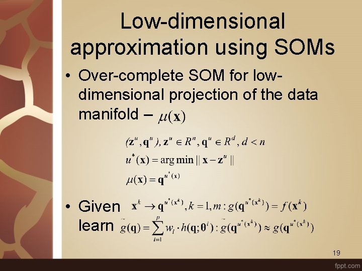
Low-dimensional approximation using SOMs • Over-complete SOM for lowdimensional projection of the data manifold – • Given learn 19

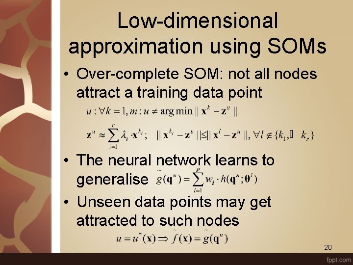
Low-dimensional approximation using SOMs • Over-complete SOM: not all nodes attract a training data point • The neural network learns to generalise • Unseen data points may get attracted to such nodes 20

Low-dimensional approximation using SOMs • The SOM projection is meaningful for data points on and around the data manifold • Extension to other data points, since is defined over , is by the use of the SOM for the projection of these points as well • The SOM-based approximation of is piecewise constant (i. e. constant over each Voronoi cell in the data space) 21

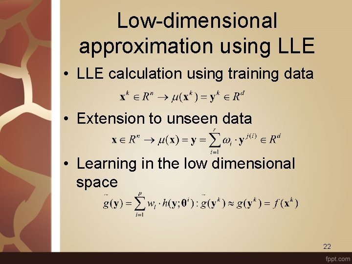
Low-dimensional approximation using LLE • LLE calculation using training data • Extension to unseen data • Learning in the low dimensional space 22

Low-dimensional approximation using LLE • The LLE projection is meaningful on and around the data manifold • The extension to other data points is a continuous extension based on the LLE projection of these points 23

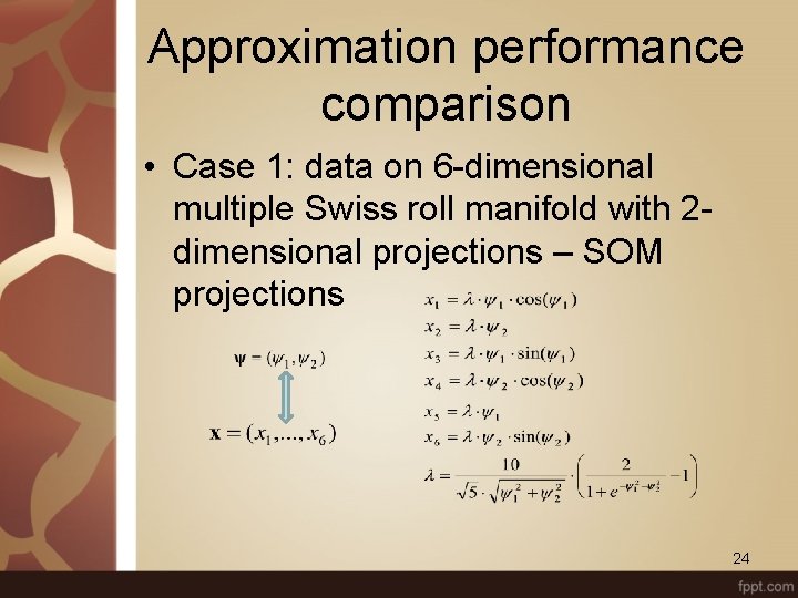
Approximation performance comparison • Case 1: data on 6 -dimensional multiple Swiss roll manifold with 2 dimensional projections – SOM projections 24

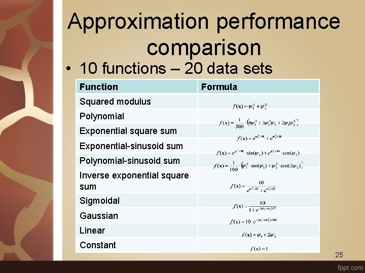
Approximation performance comparison • 10 functions – 20 data sets Function Formula Squared modulus Polynomial Exponential square sum Exponential-sinusoid sum Polynomial-sinusoid sum Inverse exponential square sum Sigmoidal Gaussian Linear Constant 25

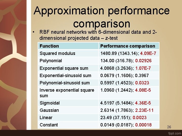
Approximation performance comparison • RBF neural networks with 6 -dimensional data and 2 dimensional projected data – z-test Function Performance comparison Squared modulus 1480. 89 (1343. 14); 4. 09 E-7 Polynomial 134. 00 (316. 78); 0. 02926 Exponential square sum 4. 0868 (3. 2636); 1. 07 E-7 Exponential-sinusoid sum 0. 0679 (1. 1606); 0. 3967 Polynomial-sinusoid sum 0. 5997 (1. 4523); 0. 0323 Inverse exponential square sum 1. 0960 (1. 2442); 4. 08 E-5 Sigmoidal 4. 5197 (5. 1484); 4. 36 E-5 Gaussian 2. 6314 (1. 7863); 2. 23 E-11 Linear 23. 49 (37. 151); 0. 0023 Constant 0. 0149 (0. 0187); 0. 00018 26

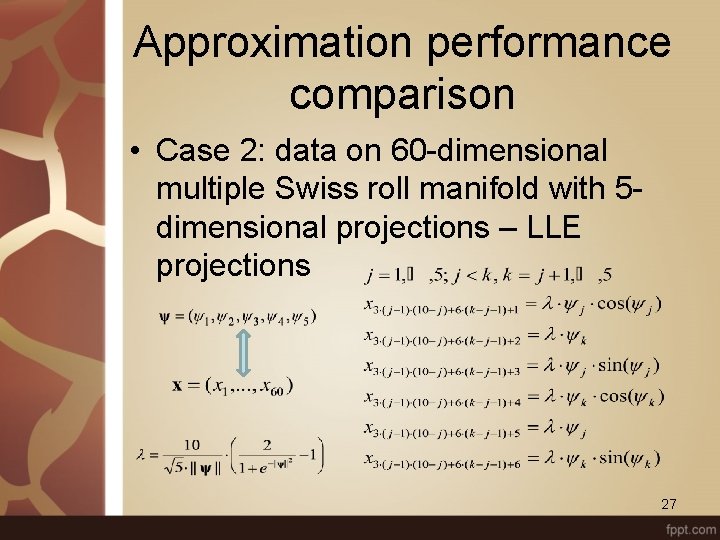
Approximation performance comparison • Case 2: data on 60 -dimensional multiple Swiss roll manifold with 5 dimensional projections – LLE projections 27

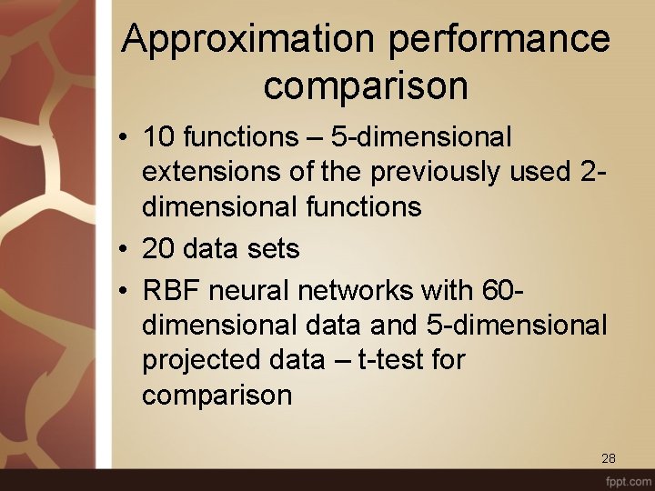
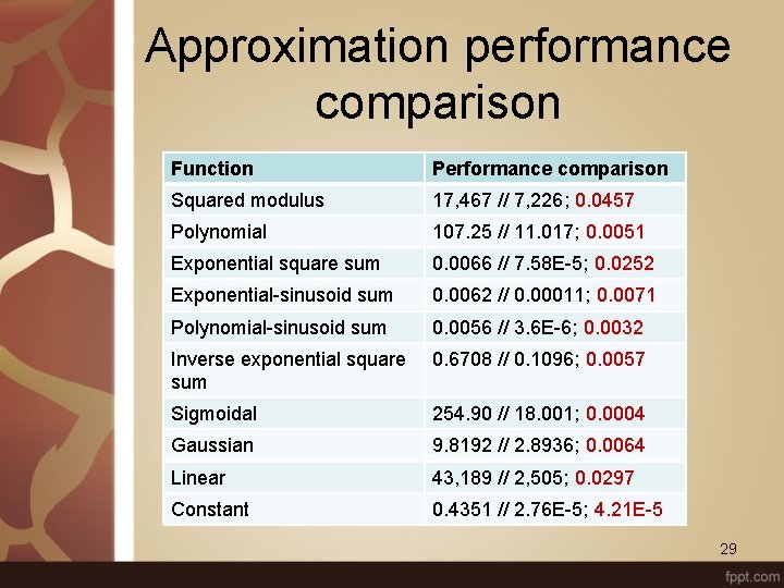
Approximation performance comparison • 10 functions – 5 -dimensional extensions of the previously used 2 dimensional functions • 20 data sets • RBF neural networks with 60 dimensional data and 5 -dimensional projected data – t-test for comparison 28

Approximation performance comparison Function Performance comparison Squared modulus 17, 467 // 7, 226; 0. 0457 Polynomial 107. 25 // 11. 017; 0. 0051 Exponential square sum 0. 0066 // 7. 58 E-5; 0. 0252 Exponential-sinusoid sum 0. 0062 // 0. 00011; 0. 0071 Polynomial-sinusoid sum 0. 0056 // 3. 6 E-6; 0. 0032 Inverse exponential square sum 0. 6708 // 0. 1096; 0. 0057 Sigmoidal 254. 90 // 18. 001; 0. 0004 Gaussian 9. 8192 // 2. 8936; 0. 0064 Linear 43, 189 // 2, 505; 0. 0297 Constant 0. 4351 // 2. 76 E-5; 4. 21 E-5 29

Extensions • The parameters of the nonlinear basis functions matter for the approximation performance of neural networks • RBF basis functions: the parameters are the centres and radii of the basis functions 30

Extensions • Support vector machine based selection of basis function parameters • Bayesian SOM learning of the data distribution in order to set the basis function parameters • Both approaches improve the approximation performance at least in a part of the considered cases 31

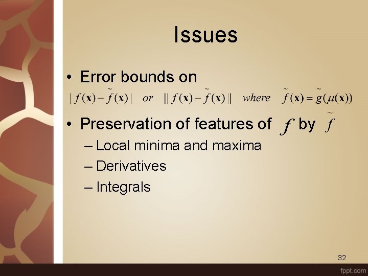
Issues • Error bounds on • Preservation of features of by – Local minima and maxima – Derivatives – Integrals 32

Conclusions • High-dimensional functions effectively defined over low dimensional manifolds can be approximated well through a combined unsupervised and supervised learning method • Manifold mapping methods matter for the preservation of features of the approximated function • Experimental analysis confirms expectations 33