Network Tools Network Simulator A network simulator is

Network Tools

Network Simulator A network simulator is a piece of software or hardware that predicts the behavior of a network, without an actual network being present.

Network Simulator (cont) Network simulators are relatively fast and inexpensive compared to the cost and time involved in setting up an entire test bed containing multiple networked computers, routers and data links, Allow engineers to test scenarios that might be particularly difficult or expensive to emulate using real hardware

simulating the effects of a sudden burst in traffic a Do. S attack on a network service test new networking protocols or changes to existing protocols in a controlled and reproducible environment With the help of simulators one can design hierarchical networks using various types of nodes like computers, hubs, bridges, routers, optical crossconnects, multicast routers, mobile units, MSAUs etc

Types of network simulators Various types of Wide Area Network (WAN) technologies like TCP, ATM, IP etc and Local Area Network (LAN) technologies like Ethernet, token rings etc. can all be simulated with a typical simulator The user can test, analyze various standard results apart from devising some novel protocol or strategy for routing etc

Types of network simulators (cont) �a network simulator must enable a user to ◦ ◦ represent a network topology, specifying the nodes on the network, the links between those nodes and the traffic between the nodes �More complicated systems may allow the user to specify everything about the protocols used to handle network traffic. �Graphical applications allow users to easily visualize the workings of their simulated environment. �Text-based applications may provide a less intuitive interface, but may permit more advanced forms of customization.

Others, such as GTNets, are programming-oriented, providing a programming framework that the user then customizes to create an application that simulates the networking environment to be tested.

Examples Ns 2 - Command based Opnet- Graphical OMNET++ Qual. Net Glomo. Sim

� OPNET solutions address application performance management; network planning, engineering, and operations; and network R&D. � OPNET solutions for Network engineering, operations, and planning include the following ◦ ◦ ◦ IT Guru Network Planner helps enterprises plan their network for new applications or technologies. SP Guru Network Planner and SP Guru Transport Planner optimize service provider network designs for capacity, cost, Qo. S, and survivability. Sentinel is OPNET's network configuration auditing solution and it is used to ensure network integrity, security, and policy compliance. Net. Mapper complements OPNET's Sentinel and Guru solutions by automatically creating content-rich network diagrams in Microsoft Visio format. OPNET n. Compass, a software solution for the NOC, enables operators to visualize real-time network topology, traffic, events, and status in a single view. � OPNET Modeler, a network modeling and simulation software solution, is one of OPNET's flagship solutions and also its oldest product

Glo. Mo. Sim �Global Mobile Information System Simulator (Glo. Mo. Sim) is a network protocol simulation software that simulates wireless and wired network systems. �Glo. Mo. Sim is designed using the parallel discrete event simulation capability provided by Parsec, a parallel programming language. �Glo. Mo. Sim currently supports protocols for a purely wireless network. �It uses the Parsec compiler to compile the simulation protocols.

Glo. Mo. Sim

NS-2 �ns was built in C++ and provides a simulation interface through OTcl, an object-oriented dialect of Tcl. �The user describes a network topology by writing OTcl scripts, and then the main ns program simulates that topology with specified parameters.

System Model A representation of the system to be used / studied in place of the actual system Allows us to study a system without actually building it (which, as we discussed previously, could be very expensive and time-consuming to do) �Physical Model A physical representation of the system (often scaled down) that is actually constructed Tests are then run on the model and the results used to make decisions about the system 13

System Model �Mathematical Model � Representing the system using logical and mathematical relationships � Simple ex: d = vot + ½ at 2 � This equation can be used to predict the distance traveled by an object at time t � However, will acceleration always be the same? � Often this model is fairly complex and defined by the entities and events � However, in order to be useful, the model must be evaluated in some way � i. e. The behavior based on the model must be determined 14

System Model Analytical evaluation If the model is not too complex we can sometimes solve it in a closed form using analytical methods One type of analytical evaluation is the Markov process (or Markov chain) Often problems that are too complex, even if they can be modeled analytically, are too computation intensive to be practical Simulation evaluation More often we need to simulate the behavior of the model 15

System Model 4 Deterministic Model • Inputs to the simulation are known values � No random variables are used � Ex: Customer arrivals to a store are monitored over a period of days and the arrival times are used as input to the simulation 4 Stochastic Model • One or more random variables are used in the simulation � Results can only be interpreted as estimates (or educated guesses) of the true behavior of the system � Quality of the simulation depends heavily on the correctness of the random data distribution > � Different situations may require different distributions Ex: Customers arrive at a store with exponentially distributed interarrival times having a mean of 5 minutes In most cases we do not know all of the input data in advance, and at least some random data is required 16

System Model �Static Model � Models a system at a single point in time, rather than over a period of time � Sometimes called Monte Carlo simulations � Model the output of a system by using input variables that could not be known exactly � Solution is a distribution of possible outcomes that can be characterized statistically �Dynamic Model � Models a system over time 17

Simple Monte Carlo Example Distribution of Charges Credit: Copyright 2008 Health Administration Press. All rights reserved.

Simple Monte Carlo Example Fifty percent of the clinic’s patients do not pay for their services, and it is equally likely that they will pay or not pay. • The payment per patient is modeled by: Probability of payment × Charges/patient = Payment/patient • A deterministic solution to this problem would be: Credit: Copyright 2008 Health Administration Press. All rights reserved.

Simple Monte Carlo Example Payment Distribution Credit: Copyright 2008 Health Administration Press. All rights reserved.

Simple Monte Carlo Example The Flaw of Averages On average each patient pays $35. However: Fifty percent of the patients pay nothing. A small percentage pay as much as $120. No individual patient pays $35. Monte Carlo simulation can reveal hidden information and a clearer understanding of the risks and rewards of a situation or decision. Credit: Copyright 2008 Health Administration Press. All rights reserved.

System Model Approach: Event-Scheduling You might have to use this approach if you were using general-purpose languages like C/C++ or FORTRAN. Concentrate on the events and how they affect the system state. We have to help the simulation evolve over time by keeping track of every event in increasing order of time of occurrence. This gets to be a bookkeeping hassle.

A Simple Processing System Arriving Blank Parts • General intent: § § • Machine (Server) 7 6 5 Queue (FIFO) 4 Departing Finished Parts Part in Service Estimate expected production Waiting time in queue, queue length, proportion of time machine is busy Time units § § Can use different units in different places … must declare Be careful to check the units when specifying inputs Declare base time units for internal calculations, outputs Be reasonable (interpretation, round-off error)

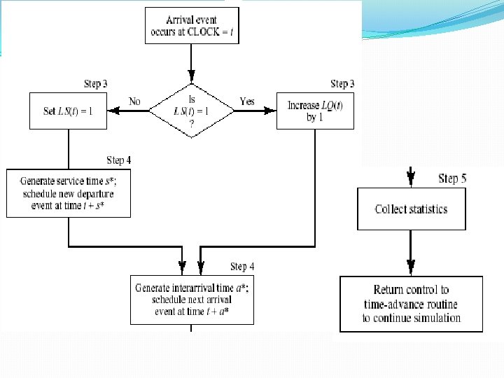
Event-Driven Simulation System state : the number of units in the system and the status of the server(busy or idle). Event : a set of circumstances that cause an instantaneous change in the state of the system. In a single-channel queueing system there are only two possible events that can affect the state of the system. the arrival event : the entry of a unit into the system the departure event : the completion of service on a unit. Simulation clock : used to track simulated time.

System Event: Arrival The arrival event occurs when a unit enters the system. The unit may find the server either idle or busy. Idle : the unit begins service immediately Busy : the unit enters the queue for the server. Arrival Event Unit enters service No Server busy? Yes Unit enters queue for service

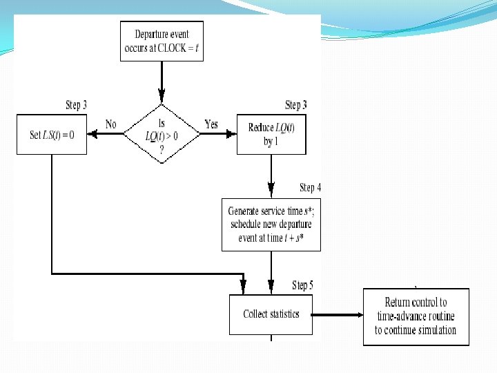
System Event: Departure If a unit has just completed service, the simulation proceeds in the manner shown in the flow diagram of Figure 2. 2. Note that the server has only two possible states : it is either busy or idle. Departure Event Begin server idle time No Another unit waiting? Yes Remove the waiting unit from the queue Begin servicing the unit

Analysis of M/M/1, M/M/c, and M/M/c/c

AGENDA Markov Chain Basic Queueing Analysis of M/M/1 Analysis of M/M/c/c

Markov Chain is a random process with the property that the next state depends only on the current state Transition probabilities Pij Transition probability matrix P=[Pij]

Example of Markov Chain State: If the weather in Hawaii today is known to be sunny, it can be represented by a vector x(0) = [1 0] That is “sunny” entry is 100% and “rainy” entry is 0% Probability Model: Let the weather model be represented by a transition matrix 0. 1 0. 9 0. 5

What do we know about tomorrow’s weather? The weather on day 1 can be predicted by Interpretation? ? There is a 90% chance that tomorrow will also be sunny 90% 10%

What about…. Can also repeat the same procedure: ? 86% 14%

In general, what’s the weather like in Hawaii? We need to find the “Steady State Probability vector” That is unchanged by P 83. 3% 16. 7%

Basic Queueing Model Buffer Server(s) Departures Arrivals Queued In Service A queue models any service station with: One or multiple servers A waiting area or buffer Customers arrive to receive service A customer that upon arrival does not find a free server is waits in the buffer 2 -36

Characteristics of a Queue b m Number of servers m: one, multiple, infinite Buffer size b Service discipline (scheduling): FCFS, LCFS, Processor Sharing (PS), etc Arrival process Service statistics 2 -37

Arrival Process : interarrival time between customers n and n+1 is a random variable is a stochastic process Interarrival times are identically distributed and have a common mean is called the arrival rate 2 -38

Service-Time Process : service time of customer n at the server is a stochastic process Service times are identically distributed with common mean is called the service rate M For packets, are the service times really random? 2 -39

Queue Descriptors Generic descriptor: A/B/m/k A denotes the arrival process For Poisson arrivals we use M (for Markovian) B denotes the service-time distribution M: exponential distribution D: deterministic service times G: general distribution m is the number of servers k is the max number of customers allowed in the system – either in the buffer or in service k is omitted when the buffer size is infinite 2 -40

Queue Descriptors: Examples M/M/1: Poisson arrivals, exponentially distributed service times, one server, infinite buffer M/M/m: same as previous with m servers M/M/m/m: Poisson arrivals, exponentially distributed service times, m server, no buffering M/G/1: Poisson arrivals, identically distributed service times follows a general distribution, one server, infinite buffer */D/∞ : A constant delay system 2 -41

M/M/1 Queue �Customers arrive according to a Poisson of rate so the interarrival times are iid exponential RV’s with mean 1/ �Service times are iid exponential RV’s with mean 1/ and are independent of the interarrival time �Single-Server system �Queue size is infinite

Required Concept: Global Balance Equations Markov chain with infinite number of states Global Balance Equations (GBE) is the frequency of transitions from j to i 3 -43

Analysis of M/M/1 0 2 1 . . . j j+1 Global Balance equation for steady-state probabilities are P 0 = P 1 (1) ( + )Pj = Pj -1 + Pj+1 ; j = 1, 2, 3… A steady state solution exists when = <1 Rewriting second part of (2) Pj - Pj+1 = Pj-1 - Pj ; (2) j = 1, 2, 3… (3)

Analysis of M/M/1 (cont) From (1) it is easy to see that P 1 - P 2 = 0 (4) Thus (3) becomes Pj-1 = Pj-1 ; j = 1, 2, 3… By induction Pj = j P 0 We obtain P 0 by noting that sum of probabilities = 1 where the series converges if and only if < 1 Pj = (1 – ) j ; j = 1, 2, 3… (5)

Analysis of M/M/1 (cont 1) Note: The condition must be met if the system is to be stable. That is N(t) does not grow. The mean number of customers in the system is given by Using (6) together with Little’s formula, the mean delay in the system is

Analysis of M/M/1 (cont 1) The mean waiting time in queue is given by By using Little’s formula, the mean number of customers in the queue is The server utilization is given by

M/M/1: Performance Metrics E[N] 0. 5 1

Multi-Server Systems: M/M/c 1 0 2 2 . . . C-2 C-1 (c-1) C c C+1 . . . j j+1 c c Arrival occurs at a rate of Departure rate is k when k servers are busy When k servers are busy, then the time until the next departure is given by X = min( 1, 2, …, k), where i are iid exponential RV’s with parameter . Then, P[X > t] = P[min ( 1, 2, …, k) > t] = P[ 1>t] P[ 2>t] … P[ k>t] = e-k t Thus the average time until the next departure is 1/k (1) (2)

Analysis of M/M/c From the general solution for birth-and-death processes, the probabilities of the first c states are obtained from the following recursion: The probabilities for states equal to or greater than c are obtained from the following recursion:

Analysis of M/M/c (cont 1) Finally, P 0 is obtained from the normalization condition: The system is stable if < 1 or < c The final form of P 0 is (6) The probability that an arriving customer finds all servers busy is

Analysis of M/M/c (cont 2) The probability in (8) is called ERLANG C formula and is denoted by C(c, a): The mean number of customers in the queue is given by: The mean waiting time is found from Little’s formula:

Analysis of M/M/c (cont 3) The mean total time in the system is E[T] = E[W] + E[ ] = E[W] + 1/ (12) Finally, the mean number in the system is found from Little’s formula: E[N] = E[T] = E[Nq] +a (13)

What are example of M/M/c/c? 1 0 2 2 . . . C-2 C-1 (c-1) C c What are the systems that use M/M/c/c? Verify for yourself that: The probability of blocking or Pc is called the Erlang B formula