Network Models 1 Context Mathematical programming Linear programming

Network Models 1

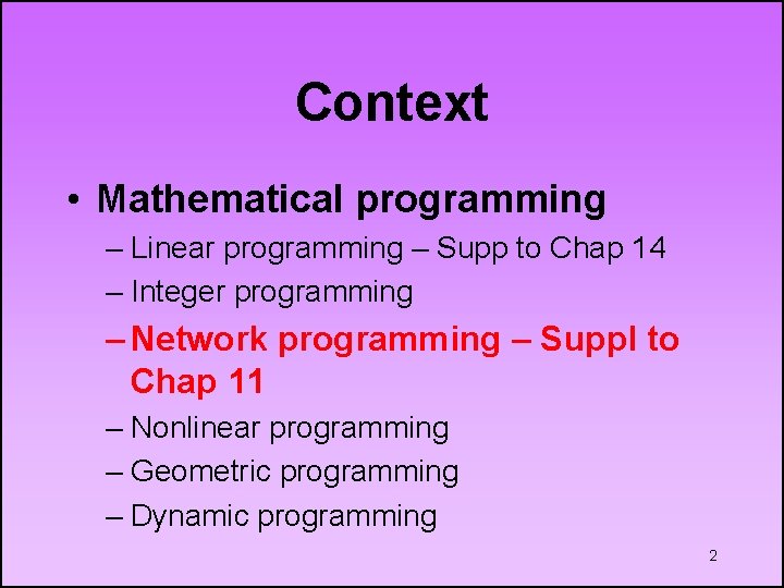
Context • Mathematical programming – Linear programming – Supp to Chap 14 – Integer programming – Network programming – Suppl to Chap 11 – Nonlinear programming – Geometric programming – Dynamic programming 2

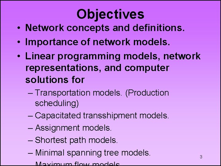
Objectives • Network concepts and definitions. • Importance of network models. • Linear programming models, network representations, and computer solutions for – Transportation models. (Production scheduling) – Capacitated transshipment models. – Assignment models. – Shortest path models. – Minimal spanning tree models. 3

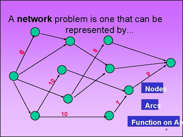
6 8 A network problem is one that can be represented by. . . 10 9 7 Nodes Arcs 10 Function on Arc 4

6. 1 Introduction • The importance of network models – Many business problems lend themselves to a network formulation. – Optimal solutions of network problems are guaranteed integer solutions, because of their special mathematical structures. No special restrictions are needed to ensure integrality – Network problems can be efficiently solved 5 fast by compact algorithms due to their

6. 1 Introduction, Cont’d – WINQSB provides the specialized algorithms necessary to get fast solutions – These models can be solved as LP models within SOLVER say but solutions could take some time for large models 6

• Network Terminology – Flow : the amount sent from node i to node j, over an arc that connects them. The following notation is used: Xij = amount of flow Uij = upper bound of the flow Lij = lower bound of the flow – Directed/undirected arcs : when flow is allowed in one direction the arc is directed (marked by an arrow). When flow is allowed in two directions, the arc is undirected (no arrows). 7

• Path / Connected nodes – Path : a collection of arcs formed by a series of adjacent nodes. – The nodes are said to be connected if there is a path between them. • Cycles / Trees / Spanning Trees – Cycle : a path starting at a certain node and returning to the same node without using any arc twice. – Tree : a series of nodes that contain no cycles. – Spanning tree : a tree that connects all the 8

Network models vs. Linear programming models • Every network model has an underlying linear programming model • For every node there is exactly one constraint • For every arc there is one decision variable Xij, where i is the starting node and j is the ending node 9

6. 2 The Transportation Problem Transportation problems arise when a cost-effective pattern is needed to ship items from origins that have limited supply to destinations that have demand for the goods. 10

• Problem definition – There are m sources. Source i has a supply capacity of Si. – There are n destinations. The demand at destination j is D j. – Objective: Minimize the total shipping cost of supplying the 11

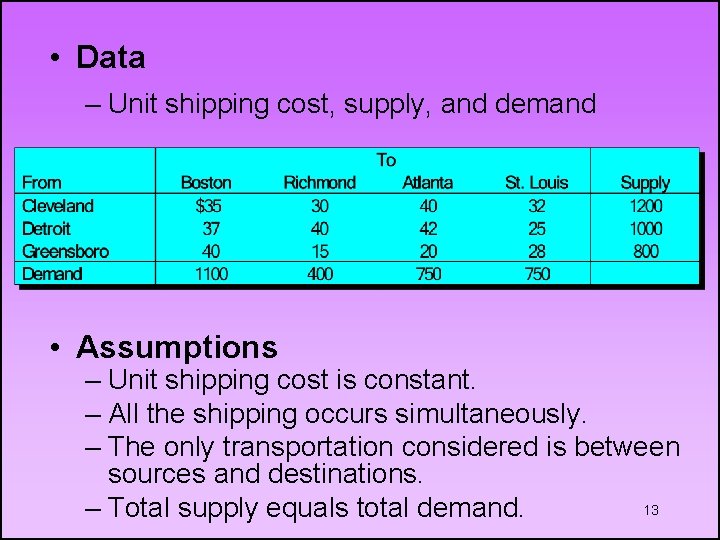
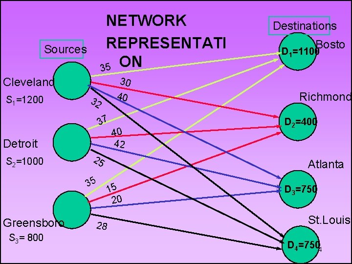
CARLTON PHARMACEUTICALS • Carlton Pharmaceuticals supplies drugs and other medical supplies. • It has three plants in: Cleveland, Detroit, Greensboro. • It has four distribution centers in: Boston, Richmond, Atlanta, St. Louis. • Management at Carlton would like to ship cases of a certain vaccine as economically as 12 possible.

• Data – Unit shipping cost, supply, and demand • Assumptions – Unit shipping cost is constant. – All the shipping occurs simultaneously. – The only transportation considered is between sources and destinations. 13 – Total supply equals total demand.

NETWORK REPRESENTATI ON 35 Sources Cleveland S 1=1200 40 32 Detroit S 3= 800 40 42 25 35 Greensboro Bosto D 1=1100 n 30 37 S 2=1000 Destinations 28 Richmond D 2=400 Atlanta 15 20 D 3=750 St. Louis D 4=750 14

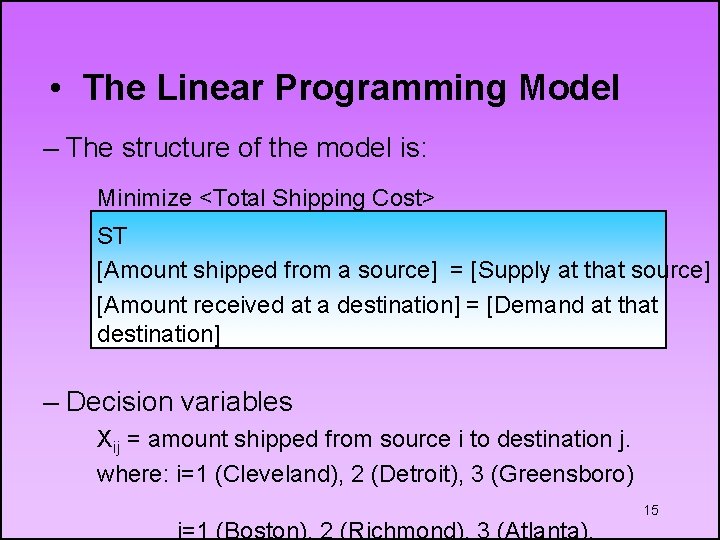
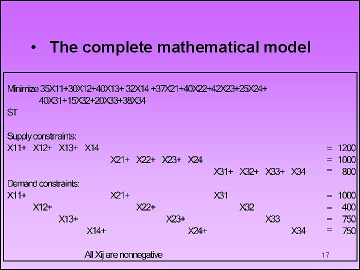
• The Linear Programming Model – The structure of the model is: Minimize <Total Shipping Cost> ST [Amount shipped from a source] = [Supply at that source] [Amount received at a destination] = [Demand at that destination] – Decision variables Xij = amount shipped from source i to destination j. where: i=1 (Cleveland), 2 (Detroit), 3 (Greensboro) j=1 (Boston), 2 (Richmond), 3 (Atlanta), 15

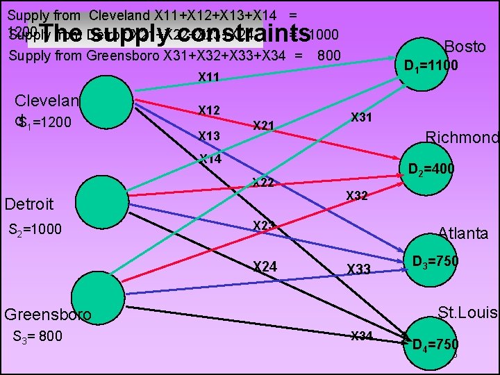
Supply from Cleveland X 11+X 12+X 13+X 14 = 1200 Supply from Detroit X 21+X 22+X 23+X 24 = 1000 Supply from Greensboro X 31+X 32+X 33+X 34 = 800 The supply constraints Bosto D 1=1100 n X 11 Clevelan d. S 1=1200 X 12 X 13 X 21 X 31 Richmond X 14 X 22 Detroit S 2=1000 D 2=400 X 32 X 23 X 24 Atlanta X 33 St. Louis Greensboro S 3= 800 D 3=750 X 34 D 4=750 16

• The complete mathematical model = = = = 17

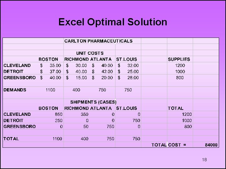
Excel Optimal Solution 18

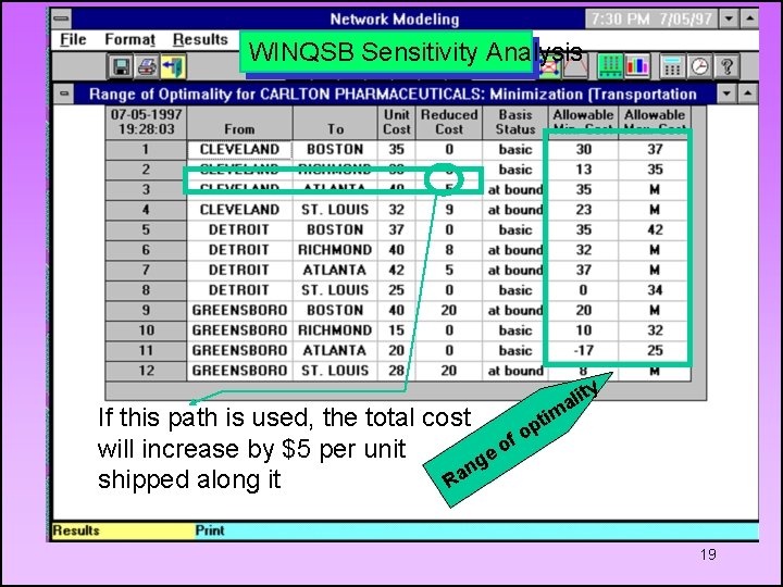
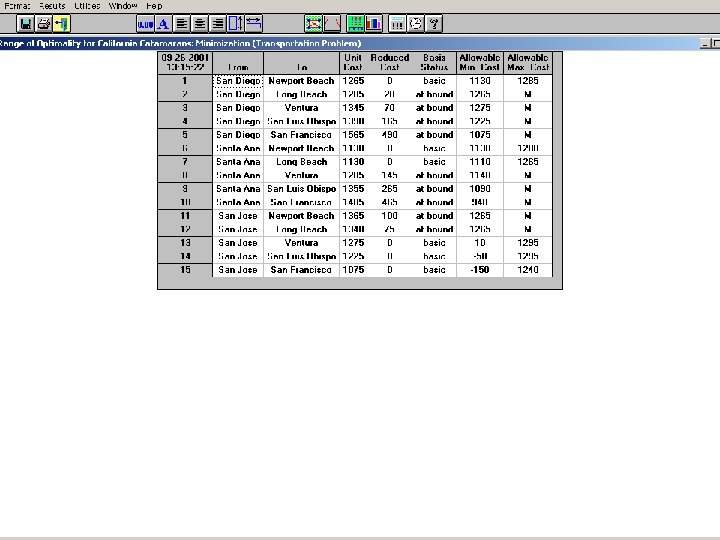
WINQSB Sensitivity Analysis lity a m If this path is used, the total cost ti p fo o will increase by $5 per unit ge n shipped along it Ra 19

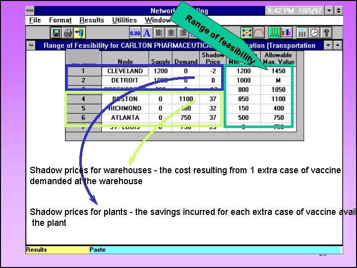
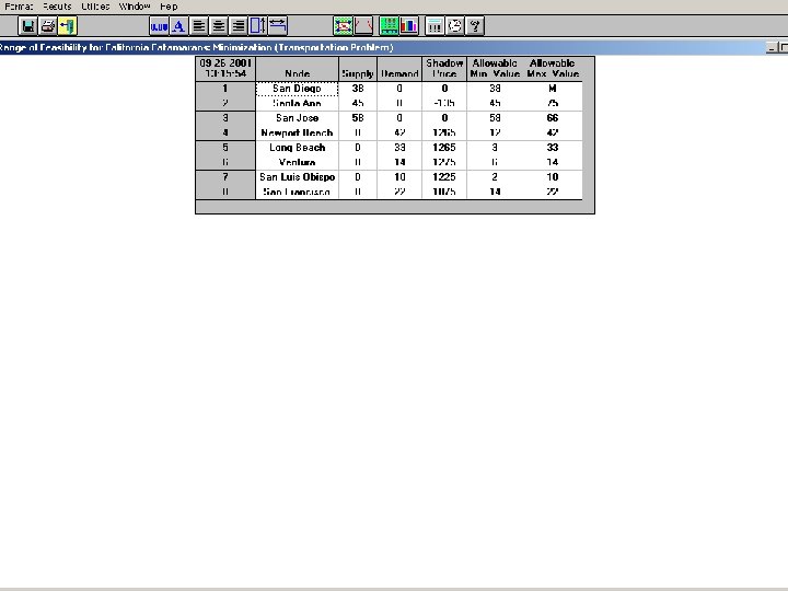
Ra ng e of fea sib ilit y Shadow prices for warehouses - the cost resulting from 1 extra case of vaccine demanded at the warehouse Shadow prices for plants - the savings incurred for each extra case of vaccine availa the plant 20

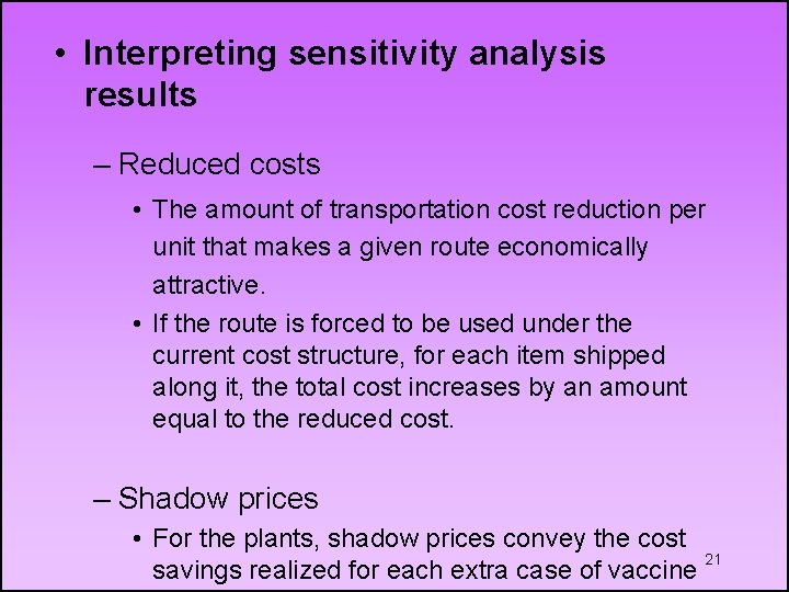
• Interpreting sensitivity analysis results – Reduced costs • The amount of transportation cost reduction per unit that makes a given route economically attractive. • If the route is forced to be used under the current cost structure, for each item shipped along it, the total cost increases by an amount equal to the reduced cost. – Shadow prices • For the plants, shadow prices convey the cost 21 savings realized for each extra case of vaccine

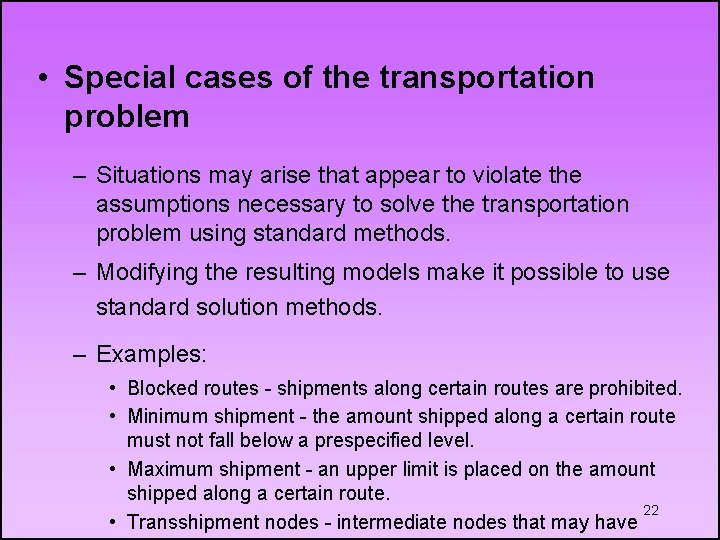
• Special cases of the transportation problem – Situations may arise that appear to violate the assumptions necessary to solve the transportation problem using standard methods. – Modifying the resulting models make it possible to use standard solution methods. – Examples: • Blocked routes - shipments along certain routes are prohibited. • Minimum shipment - the amount shipped along a certain route must not fall below a prespecified level. • Maximum shipment - an upper limit is placed on the amount shipped along a certain route. 22 • Transshipment nodes - intermediate nodes that may have

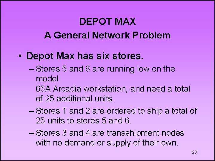
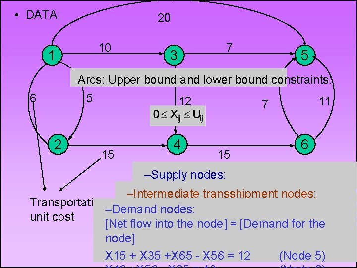
DEPOT MAX A General Network Problem • Depot Max has six stores. – Stores 5 and 6 are running low on the model 65 A Arcadia workstation, and need a total of 25 additional units. – Stores 1 and 2 are ordered to ship a total of 25 units to stores 5 and 6. – Stores 3 and 4 are transshipment nodes with no demand or supply of their own. 23

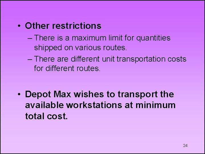
• Other restrictions – There is a maximum limit for quantities shipped on various routes. – There are different unit transportation costs for different routes. • Depot Max wishes to transport the available workstations at minimum total cost. 24

• DATA: 20 10 1 7 3 5 Arcs: Upper bound and lower bound constraints: 6 5 2 12 15 4 11 7 15 –Supply nodes: Network presentation 6 Net flow outtransshipment of the node] =nodes: [Supply at the –Intermediate Transportation X 12 flow + X 13 - X 21 == [Total 10 flow into( [Total out + of. X 15 the node] –Demand nodes: unit cost X 21 X 24 - X 12= [Demand = 15 (Node [Net. X 34+X 35 flow into+ the node] for(Node the = X 13 3) 2 node] X 46 = X 24 + X 34 (Node 4) 25 X 15 + X 35 +X 65 - X 56 = 12 (Node 5)

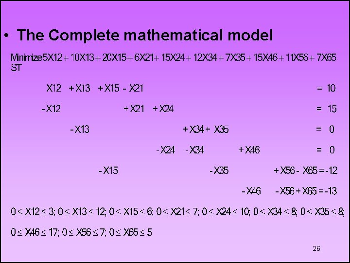
• The Complete mathematical model 26

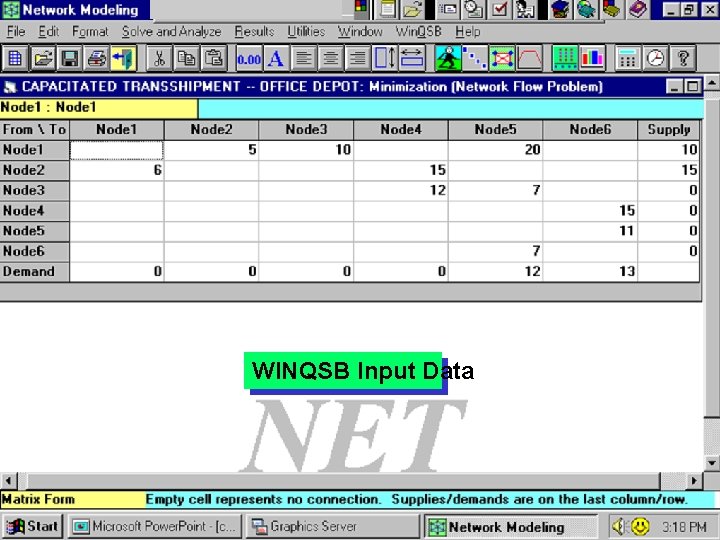
WINQSB Input Data 27

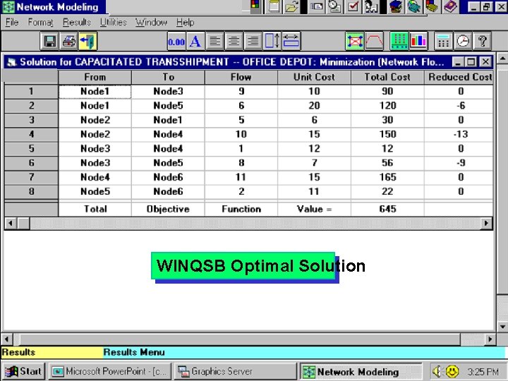
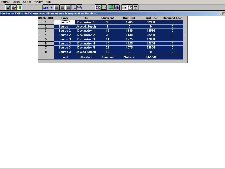
WINQSB Optimal Solution 28

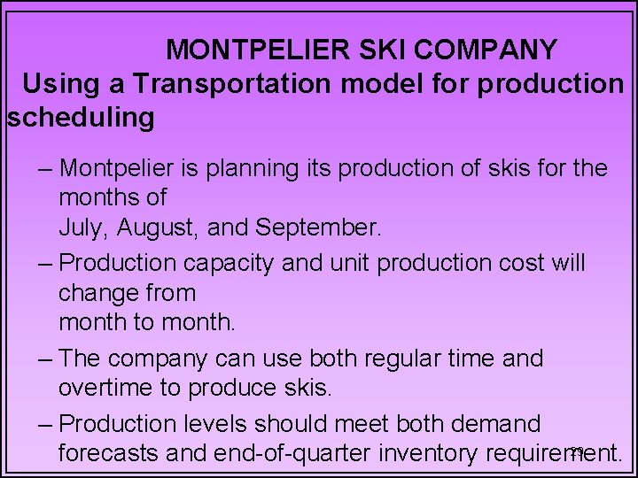
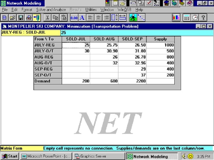
MONTPELIER SKI COMPANY Using a Transportation model for production scheduling – Montpelier is planning its production of skis for the months of July, August, and September. – Production capacity and unit production cost will change from month to month. – The company can use both regular time and overtime to produce skis. – Production levels should meet both demand 29 forecasts and end-of-quarter inventory requirement.

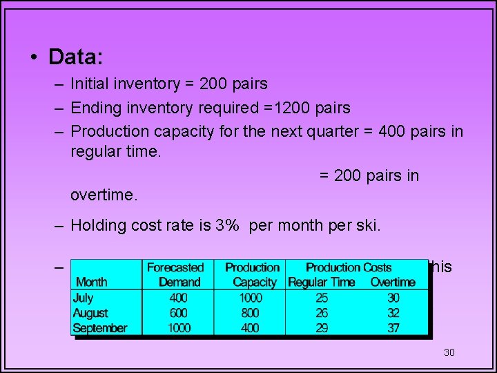
• Data: – Initial inventory = 200 pairs – Ending inventory required =1200 pairs – Production capacity for the next quarter = 400 pairs in regular time. = 200 pairs in overtime. – Holding cost rate is 3% per month per ski. – Production capacity, and forecasted demand for this quarter (in pairs of skis), and production cost per unit (by months) 30

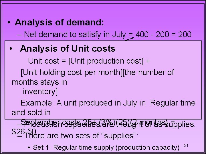
• Analysis of demand: – Net demand to satisfy in July = 400 - 200 = 200 pairs Initial inventory • Analysis of Unit costs Unit cost = [Unit production cost] + – Net demand in August = 600 [Unit holding cost per month][the number of – Net demand 1000 + house 1200 inventory = 2200 Forecasted = demand. In months stays in in September pairs inventory] Example: A unit produced in July in Regular time • and Analysis sold in of Supplies: 25+ (3%)(25)(2 = –September Productioncosts capacities are thoughtmonths) of as supplies. $26. 50 – There are two sets of “supplies”: • Set 1 - Regular time supply (production capacity) 31

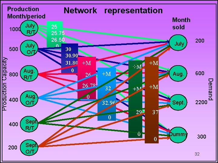
Production Month/period July 1000 R/T 800 400 200 July O/T Aug. R/T Aug. O/T Sept. R/T Sept. O/T 25 25. 75 26. 50 0 30 30. 90 31. 80 +M 0 Month sold July +M 26. 78 32 0 +M +M 0 0 Aug. 600 Sept. 2200 Dummy 300 +M 32. 96 29 200 Demand Production Capacity 500 Network representation 37 0 32

Source: July production in R/T Source: Aug. production in O/T Destination: July‘s demand. Destination: Sept. ’s demand Unit cost= $25 (production) 32+(. 03)(32)=$32. 96 Unit cost =Production+one month holding co 33

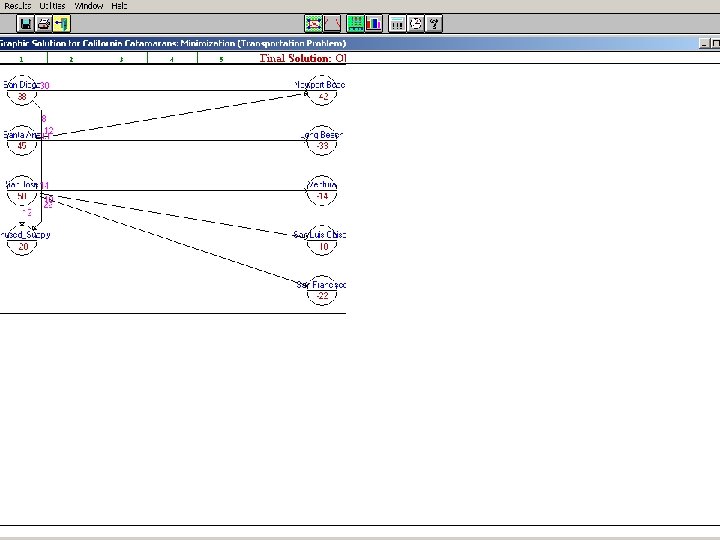
34

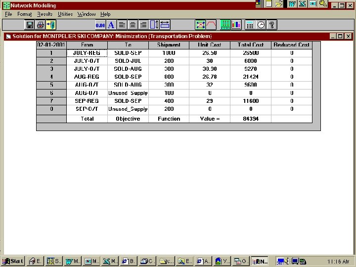
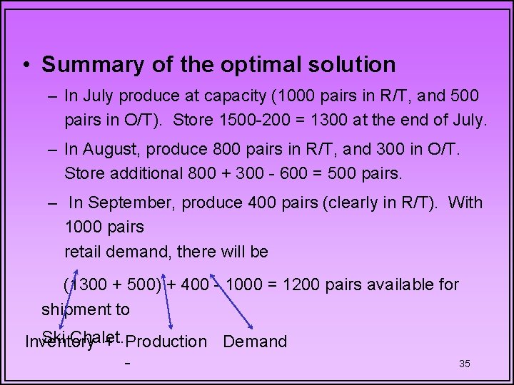
• Summary of the optimal solution – In July produce at capacity (1000 pairs in R/T, and 500 pairs in O/T). Store 1500 -200 = 1300 at the end of July. – In August, produce 800 pairs in R/T, and 300 in O/T. Store additional 800 + 300 - 600 = 500 pairs. – In September, produce 400 pairs (clearly in R/T). With 1000 pairs retail demand, there will be (1300 + 500) + 400 - 1000 = 1200 pairs available for shipment to Ski Chalet Inventory +. Production Demand - 35

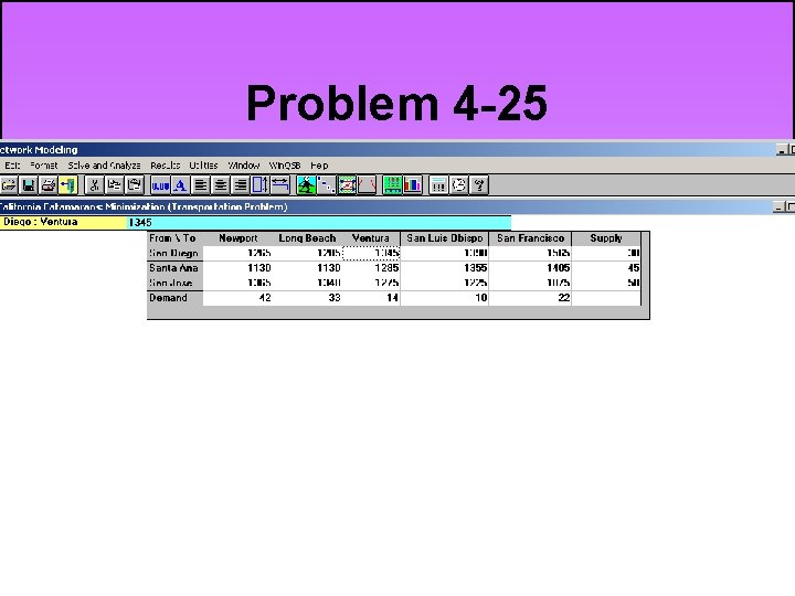
Problem 4 -25 36

37

38

39

40

6. 3 The Assignment Problem • Problem definition – m workers are to be assigned to m jobs – A unit cost (or profit) Cij is associated with worker i performing job j. – Minimize the total cost (or maximize the total profit) of assigning workers to job so that each worker is assigned a job, and each job is performed. 41

BALLSTON ELECTRONICS • Five different electrical devices produced on five production lines, are needed to be inspected. • The travel time of finished goods to inspection areas depends on both the production line and the inspection area. • Management wishes to designate a separate inspection area to inspect the products such 42 that the total travel time is minimized.

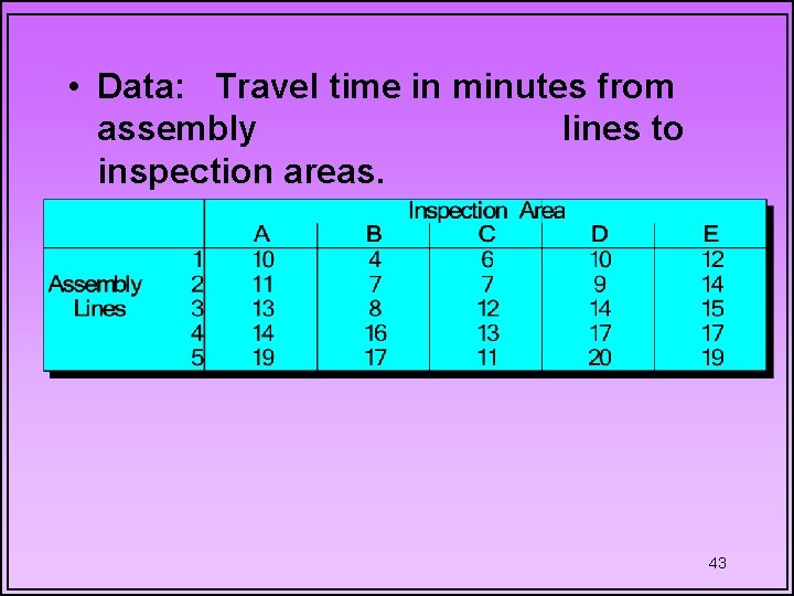
• Data: Travel time in minutes from assembly lines to inspection areas. 43

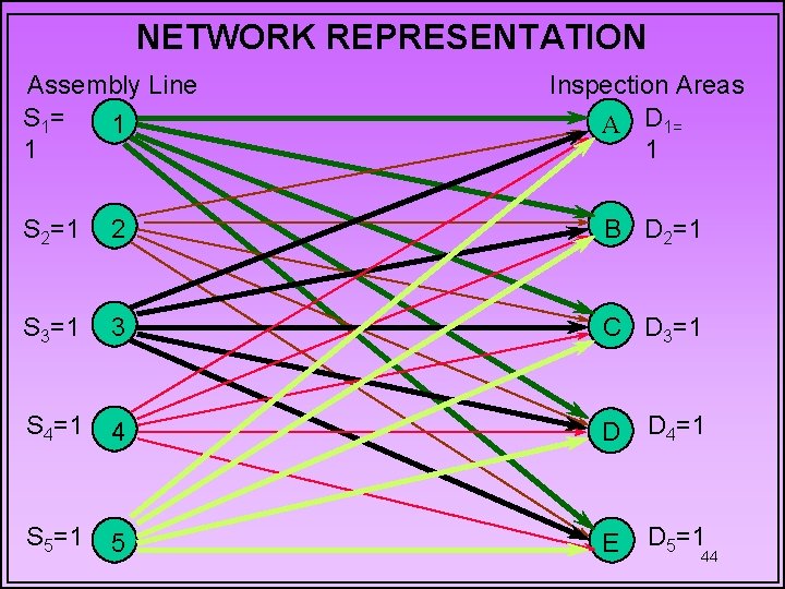
NETWORK REPRESENTATION Assembly Line S 1= 1 1 Inspection Areas A D 1= 1 S 2=1 2 B D 2=1 S 3=1 3 C D 3=1 S 4=1 4 D D 4=1 S 5=1 5 E D 5=1 44

• Assumptions and restrictions – The number of workers equals the number of jobs. – Given a balanced problem, each worker is assigned exactly once, and each job is performed by exactly one worker. – For an unbalanced problem “dummy” workers (in case there are more jobs than workers), or “dummy” jobs (in case there are more workers than jobs) are added to balance the problem. 45

• Computer solutions – A complete enumeration is not efficient even for moderately large problems (with m=8, m! > 40, 000 is the number of assignments to enumerate). – The Hungarian method provides an efficient solution procedure. • Special cases – A worker is unable to perform a particular job. – A worker can be assigned to more than one job. 46 – A maximization assignment problem.

6. 5 The Shortest Path Problem • For a given network find the path of minimum distance, time, or cost from a starting point, the start node, to a destination, the terminal node. • Problem definition – There are n nodes, beginning with start node 1 and ending with terminal node n. 47 – Bi-directional arcs connected nodes i

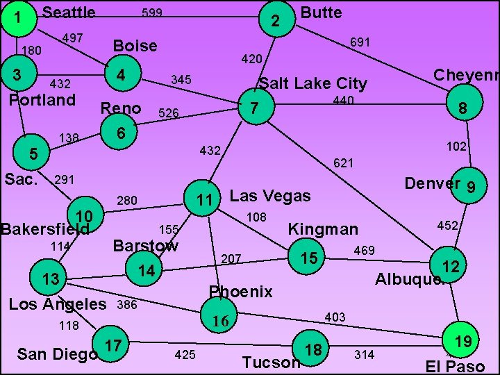
Fairway Van Lines Determine the shortest route from Seattle to El Paso over the following network highways. 48

1 Seattle 180 3 497 138 2 4 Reno 6 420 345 440 7 621 108 155 13 Los Angeles Barstow 14 207 469 15 12 Albuque. 403 16 118 425 452 Kingman Phoenix 386 17 Denver 9 11 Las Vegas 280 114 8 102 432 10 Bakersfield Cheyenn Salt Lake City 526 291 San Diego Butte 691 Boise 432 Portland 5 Sac. 599 Tucson 18 314 19 49 El Paso

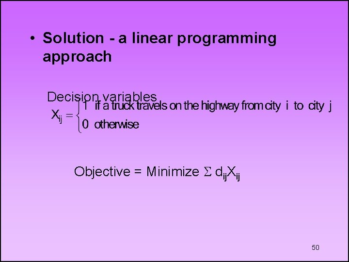
• Solution - a linear programming approach Decision variables Objective = Minimize S dij. Xij 50

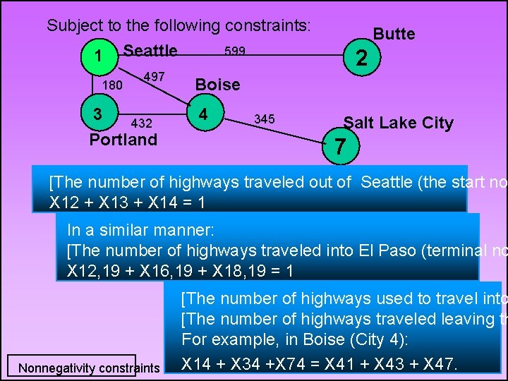
Subject to the following constraints: 599 1 Seattle 180 497 3 432 Portland Butte 2 Boise 4 345 Salt Lake City 7 [The number of highways traveled out of Seattle (the start no X 12 + X 13 + X 14 = 1 In a similar manner: [The number of highways traveled into El Paso (terminal no X 12, 19 + X 16, 19 + X 18, 19 = 1 Nonnegativity constraints [The number of highways used to travel into [The number of highways traveled leaving th For example, in Boise (City 4): X 14 + X 34 +X 74 = X 41 + X 43 + X 47. 51

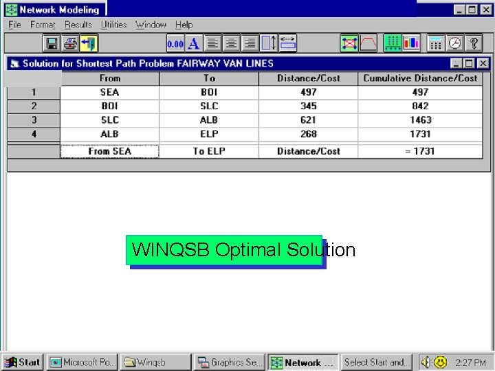
WINQSB Optimal Solution 52

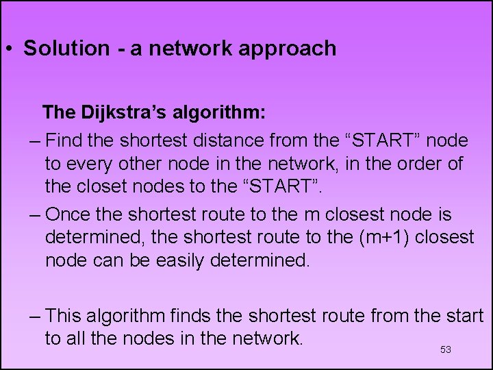
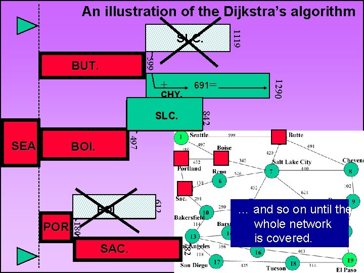
• Solution - a network approach The Dijkstra’s algorithm: – Find the shortest distance from the “START” node to every other node in the network, in the order of the closet nodes to the “START”. – Once the shortest route to the m closest node is determined, the shortest route to the (m+1) closest node can be easily determined. – This algorithm finds the shortest route from the start to all the nodes in the network. 53

An illustration of the Dijkstra’s algorithm SLC 599 BUT. 691= 345 = + SLC CHY. SEA. BOI BOI. + 432 = BOIBOI 612 180 497 180 POR. + 602 = SACSAC. 782 POR 1290 + 842 BUT 1119 + 420 = SLC. … and so on until the whole network is covered. 54

6. 6 The Minimal Spanning Tree • This problem arises when all the nodes of a given network must be connected to one another, without any loop. • The minimal spanning tree approach is appropriate for problems for which redundancy is expensive, or the flow along the arcs is considered 55

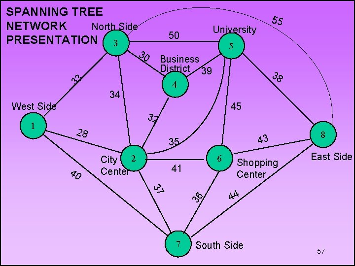
THE METROPOLITAN TRANSIT DISTRICT • The City of Vancouver is planning the development of a new light rail transportation system. • The system should link 8 residential and commercial centers. • The Metropolitan transit district needs to select the set of lines that will connect all the centers at a minimum total cost. 56

SPANNING TREE NETWORK North Side PRESENTATION 3 38 4 34 45 32 28 40 43 35 City 2 Center 6 41 37 36 1 5 Business District 39 33 West Side University 50 30 55 7 Shopping Center 8 East Side 44 South Side 57

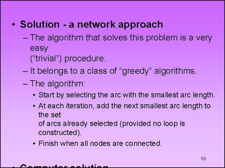
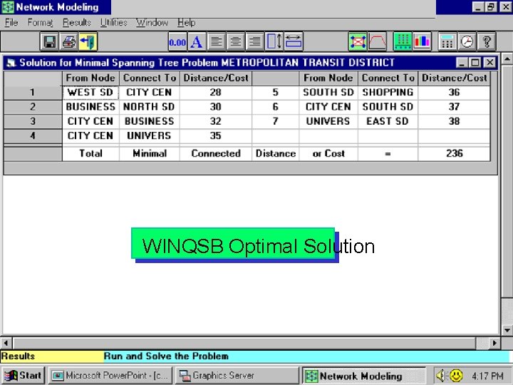
• Solution - a network approach – The algorithm that solves this problem is a very easy (“trivial”) procedure. – It belongs to a class of “greedy” algorithms. – The algorithm: • Start by selecting the arc with the smallest arc length. • At each iteration, add the next smallest arc length to the set of arcs already selected (provided no loop is constructed). • Finish when all nodes are connected. 58

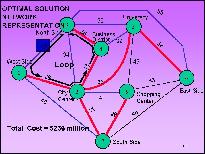
WINQSB Optimal Solution 59

OPTIMAL SOLUTION NETWORK REPRESENTATION 3 North Side 1 45 32 28 40 38 4 34 Loop 5 Business District 39 33 West Side University 50 30 55 43 35 City 2 Center 6 41 37 36 Shopping Center 8 East Side 44 Total Cost = $236 million 7 South Side 60

6. 7 The Maximal Flow Problem • The model is designed to reduce or eliminate bottlenecks between a certain starting point and some destination of a given network. • A flow travels from a single source to a single sink over arcs connecting intermediate nodes. 61 • Each arc has a capacity that cannot be

• Problem definition – There is a source node (labeled 1), from which the network flow emanates. – There is a terminal node (labeled n), into which all network flow is eventually deposited. – There are n - 2 intermediate nodes (labeled 2, 3, …, n-1), where the node inflow is equal to the node outflow. – There are capacities Cij for flow on the arc from 62 node i to node j, and capacities Cji for the opposite

The objective is to find the maximum tota out of node 1 that can flow into node n w exceeding the capacities on the arcs. 63

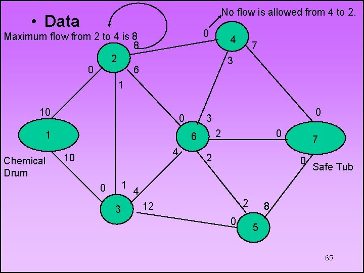
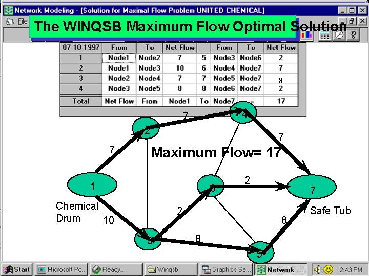
UNITED CHEMICAL COMPANY • United Chemical produces pesticides and lawn care products. • Poisonous chemicals needed for the production process are held in a huge drum. • A network of pipes and valves regulates the chemical flow from the drum to different production areas. • The safety division must plan a procedure to empty the drum as fast as possible into a safety tub in the disposal area, using the same network 64 of pipes and valves.

No flow is allowed from 4 to 2. • Data 0 Maximum flow from 2 to 4 is 8 8 2 0 6 4 7 3 1 10 0 1 Chemical Drum 2 6 4 10 1 0 3 0 2 7 0 Safe Tub 4 2 12 0 8 5 65

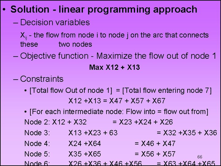
• Solution - linear programming approach – Decision variables Xij - the flow from node i to node j on the arc that connects these two nodes – Objective function - Maximize the flow out of node 1 Max X 12 + X 13 – Constraints • [Total flow Out of node 1] = [Total flow entering node 7] X 12 +X 13 = X 47 + X 57 + X 67 • [For each intermediate node: Flow into = flow out from] Node 2: X 12 + X 32 = X 23 +X 24 + X 26 Node 3: X 13 +X 23 + 63 = X 32 +X 35 + X 36 Node 4: X 24 +X 64 = X 46 + X 47 Node 5: X 35 +X 65 = X 56 + X 57 66

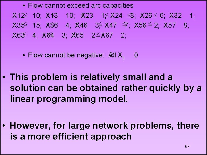
• Flow cannot exceed arc capacities X 12 10; X 13 10; X 23 1; X 24 8; X 26 6; X 32 1; X 35 15; X 36 4; X 46 3; X 47 7; X 56 2; X 57 8; X 63 4; X 64 3; X 65 2; X 67 2; • Flow cannot be negative: All Xij 0 • This problem is relatively small and a solution can be obtained rather quickly by a linear programming model. • However, for large network problems, there is a more efficient approach 67

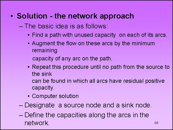
• Solution - the network approach – The basic idea is as follows: • Find a path with unused capacity on each of its arcs. • Augment the flow on these arcs by the minimum remaining capacity of any arc on the path. • Repeat this procedure until no path from the source to the sink can be found in which all arcs have residual positive capacity. • Computer solution – Designate a source node and a sink node. – Define the capacities along the arcs in the network. 68

The WINQSB Maximum Flow Optimal Solution 8 4 7 2 7 7 Maximum Flow= 17 1 6 Chemical Drum 10 2 7 2 3 8 Safe Tub 8 5 69

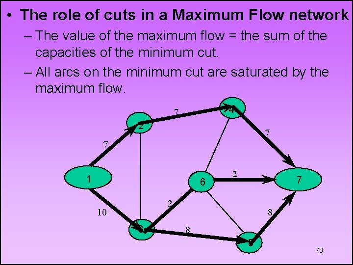
• The role of cuts in a Maximum Flow network – The value of the maximum flow = the sum of the capacities of the minimum cut. – All arcs on the minimum cut are saturated by the maximum flow. 4 7 2 7 7 1 6 2 7 2 10 3 8 8 5 70

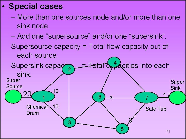
• Special cases – More than one sources node and/or more than one sink node. – Add one “supersource” and/or one “supersink”. Supersource capacity = Total flow capacity out of each source. 4 Supersink capacity = Total capacities into each 7 2 sink. Super Source 20 Super Sink 10 6 1 2 7 Chemical 10 Drum 17 Safe Tub 8 3 5 71

6. 4 The Traveling Salesman Problem • • AProblem tour begins at a home city, visits definition every city (node) in–a. There given network exactly once, and are m nodes. returns to the – Unit cost Cij is associated with utilizing arc home (i, j) city. – Find the cycle that minimizes the total cost • Therequired objective is all tothe minimize the travel to visit nodes exactly once. time/distance. 72

Complexity • • Importance: Writing of thescheduling mathematical model can be solved – Variety applications and as a solving this problem are both cumbersome (a problem with 20 traveling salesmen problem. cities – Examples: requires 500, 000 • Orderingover drill position onlinear a drill press. constraints. ) • School bus routing. • Military bombing sorties. – The problem has theoretical importance because it represents a class of difficult problems known as NP-hard problems. 73

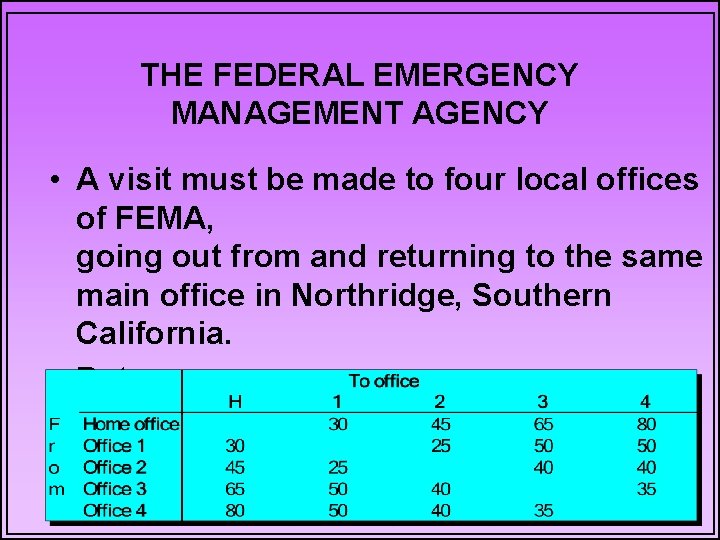
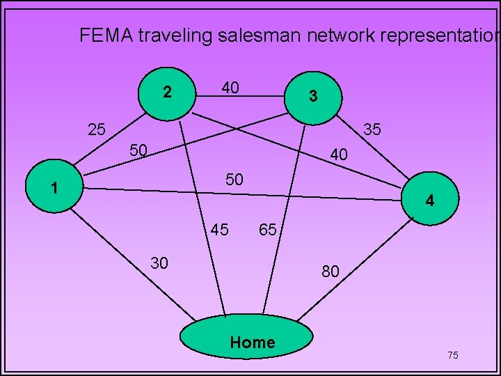
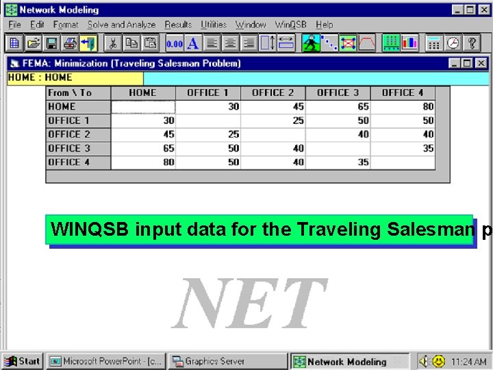
THE FEDERAL EMERGENCY MANAGEMENT AGENCY • A visit must be made to four local offices of FEMA, going out from and returning to the same main office in Northridge, Southern California. • Data Travel time between offices (minutes) 74

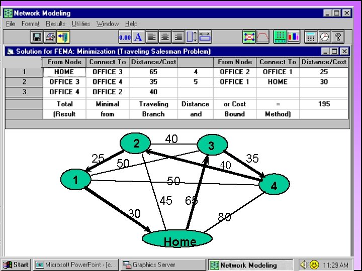
FEMA traveling salesman network representation 2 40 3 25 35 50 40 50 1 4 45 65 30 80 Home 75

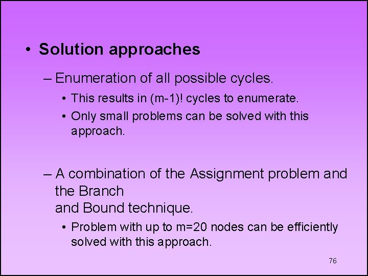
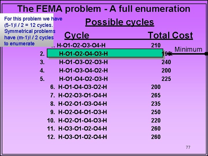
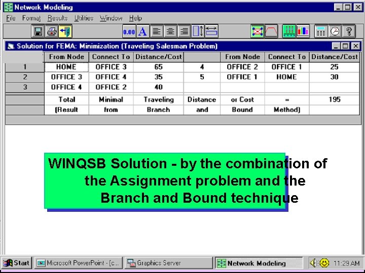
• Solution approaches – Enumeration of all possible cycles. • This results in (m-1)! cycles to enumerate. • Only small problems can be solved with this approach. – A combination of the Assignment problem and the Branch and Bound technique. • Problem with up to m=20 nodes can be efficiently solved with this approach. 76

The FEMA problem - A full enumeration For this problem we have Possible cycles (5 -1)! / 2 = 12 cycles. Symmetrical problems Cycle Total Cost have (m-1)! / 2 cycles to enumerate 2. 3. 4. 5. 1. H-O 1 -O 2 -O 3 -O 4 -H H-O 1 -O 2 -O 4 -O 3 -H H-O 1 -O 3 -O 2 -O 3 -H H-O 1 -O 3 -O 4 -O 2 -H H-O 1 -O 4 -O 2 -O 3 -H 6. H-O 1 -O 4 -O 3 -O 2 -H 7. H-O 2 -O 3 -O 1 -O 4 -H 8. H-O 2 -O 1 -O 3 -O 4 -H 9. H-O 2 -O 4 -O 1 -O 3 -H 10. H-O 2 -O 1 -O 4 -O 3 -H 11. H-O 3 -O 1 -O 2 -O 4 -H 12. H-O 3 -O 1 -O 2 -O 4 -H 210 195 240 200 225 Minimum 200 265 235 250 220 260 77

WINQSB input data for the Traveling Salesman p 78

WINQSB Solution - by the combination of the Assignment problem and the Branch and Bound technique 79

2 40 3 25 50 1 40 50 30 45 35 4 65 80 Home 80

• Special Cases – Revisiting nodes : a node can be revisited before the end of the cycle. To handle this situation: • find the shortest path from each city to any other city, • substitute the shortest path for the ”direct distance” value. • solve the traveling salesman problem with the new distances. – n-person traveling salesman problem 81 • n objects must visit m nodes, but no two objects visit

42

• Copyright ã 1998 John Wiley & Sons, Inc. All rights reserved. Reproduction or translation of this work beyond that named in Section 117 of the United States Copyright Act without the express written consent of the copyright owner is unlawful. Requests for further information should be addressed to the Permissions Department, John Wiley & Sons, Inc. The purchaser may make back-up copies for his/her own use only and not for distribution or resale. 83