Network Layer goals understand principles behind network layer

Network Layer goals: understand principles behind network layer services: routing (path selection) how a router works Postal-service mail carrier Overview: network layer services routing principle: path selection hierarchical routing IP what’s inside a router? instantiation and implementation in the Internet Routing 1

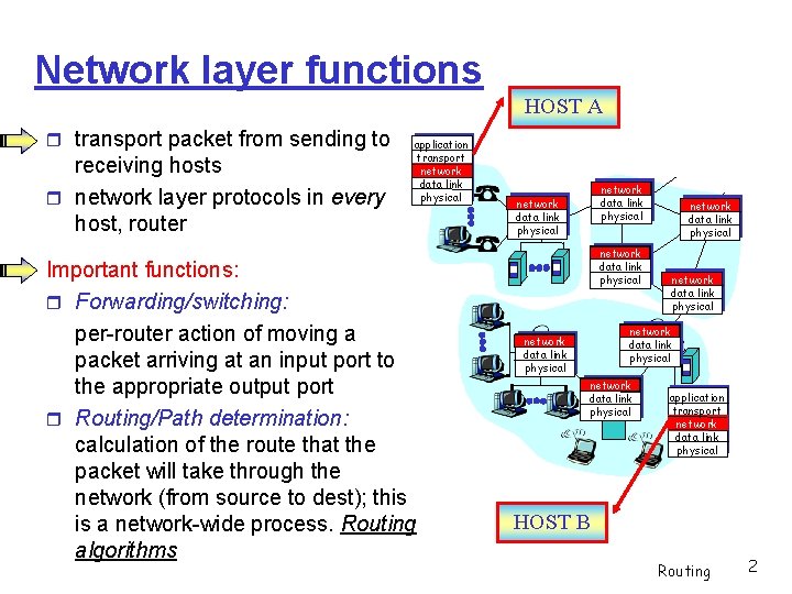
Network layer functions HOST A transport packet from sending to receiving hosts network layer protocols in every host, router application transport network data link physical Important functions: Forwarding/switching: per-router action of moving a packet arriving at an input port to the appropriate output port Routing/Path determination: calculation of the route that the packet will take through the network (from source to dest); this is a network-wide process. Routing algorithms network data link physical network data link physical application transport network data link physical HOST B Routing 2

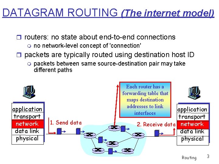
DATAGRAM ROUTING (The internet model) routers: no state about end-to-end connections no network-level concept of 'connection' packets are typically routed using destination host ID packets between same source-destination pair may take different paths application transport network data link physical Each router has a forwarding table that maps destination addresses to link interfaces 1. Send data application transport 2. Receive data network data link physical Routing 3

Routing Physical distance, link speed, monetary cost, etc. Routing protocol Goal: determine good path (sequence of routers) through network from source to destination. 5 2 A B 2 1 3 C 3 5 F 1 2 D E Graph (undirected) abstraction 1 for routing algorithms: nodes represent routers 'good' path: Lines/graph edges are typically means minimum physical links cost path link cost: delay, cost of sending a packet across link, or congestion level other definitions possible Routing 4

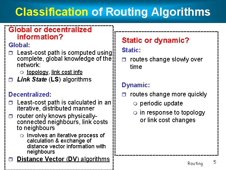
Classification of Routing Algorithms Global or decentralized information? Global: Least-cost path is computed using complete, global knowledge of the network: topology, link cost info Link State (LS) algorithms Decentralized: Least-cost path is calculated in an iterative, distributed manner router only knows physicallyconnected neighbours, link costs to neighbours Static or dynamic? Static: routes change slowly over time Dynamic: routes change more quickly periodic update in response to topology or link cost changes Involves an iterative process of calculation & exchange of distance vector information with neighbours Distance Vector (DV) algorithms Routing 5

Distance Vector Routing Algorithm iterative: continues until no nodes exchange information anymore self-terminating: no signal to stop asynchronous: nodes need not exchange info/iterate in lock step! distributed: each node communicates only with directly-attached neighbours Routing 6

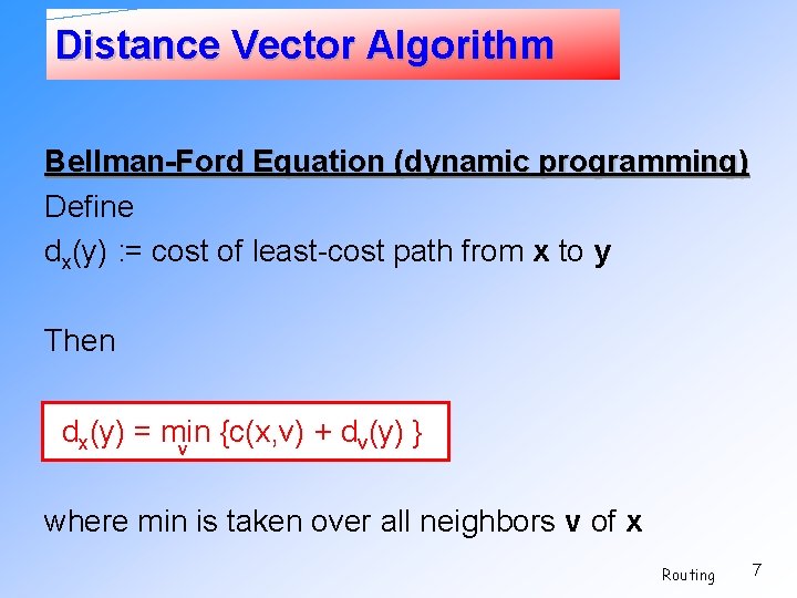
Distance Vector Algorithm Bellman-Ford Equation (dynamic programming) Define dx(y) : = cost of least-cost path from x to y Then dx(y) = min {c(x, v) + dv(y) } v where min is taken over all neighbors v of x Routing 7

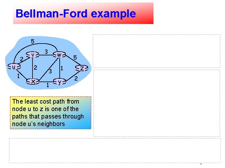
Bellman-Ford example By inspection from the graph, we can see that: 5 2 u v 2 1 x 3 w 3 1 5 z 1 y 2 The least cost path from node u to z is one of the paths that passes through node u’s neighbors dv(z) = 5, dx(z) = 3, dw(z) = 3 B-F equation says: du(z) = min { c(u, v) + dv(z), c(u, x) + dx(z), c(u, w) + dw(z) } = min {2 + 5, 1 + 3, 5 + 3} = 4 The node that arrives with the minimum cost = the next hop neighbour along the shortest path ➜ forwarding table Routing 8

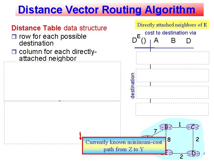
Distance Vector Routing Algorithm Calculation of values example: Node X, routing for destination Y via directly attached neighbor Z: X D (Y, Z) distance from X to = Y, via Z as next hop Directly attached neighbors of E E cost to destination via D () A B D A 1 14 5 B 7 8 5 C 6 9 4 D 4 11 2 destination Distance Table data structure row for each possible destination column for each directlyattached neighbor Z = c(X, Z) + minw{D (Y, w)} 7 B A Currently known minimum-cost 8 path from Z to Y 1 E 1 C 2 Routing. D 2 9

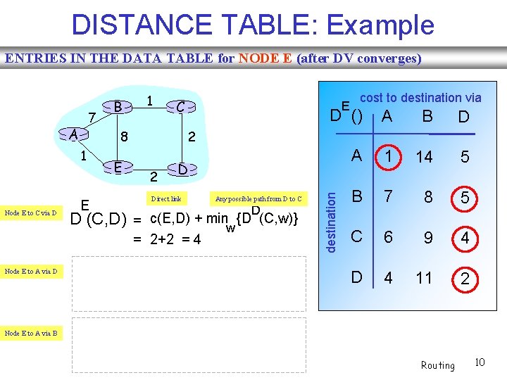
DISTANCE TABLE: Example ENTRIES IN THE DATA TABLE for NODE E (after DV converges) A C E E E 2 D () A B D A 1 14 5 B 7 8 5 C 6 9 4 D 4 11 2 D Direct link Any possible path from D to C D D (C, D) = c(E, D) + minw {D (C, w)} = 2+2 = 4 Node E to A via D cost to destination via 2 8 1 Node E to C via D 1 E D D (A, D) = c(E, D) + minw {D (A, w)} destination 7 B = 2+3 = 5 loop! Node E to A via B E B D (A, B) = c(E, B) + minw{D (A, w)} = 8+6 = 14 loop! Routing 10

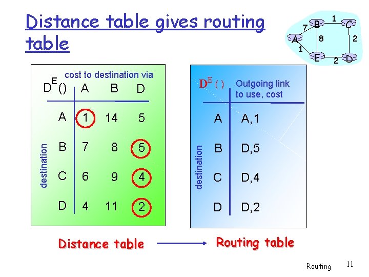
Distance table gives routing table E cost to destination via DE() B D A 1 14 5 A A, 1 B 7 8 5 B D, 5 C 6 9 4 C D, 4 D 4 11 2 D D, 2 destination A destination 1 1 2 8 E C 2 D Outgoing link to use, cost D () Distance table A 7 B Routing table Routing 11

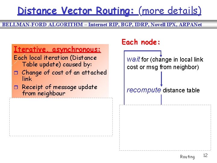
Distance Vector Routing: (more details) BELLMAN-FORD ALGORITHM – Internet RIP, BGP, IDRP, Novell IPX, ARPANet Iterative, asynchronous: Each local iteration (Distance Table update) caused by: Change of cost of an attached link Receipt of message update from neighbour Each node: wait for (change in local link cost or msg from neighbor) recompute distance table Distributed: each node notifies neighbours only when its least-cost path to any destination changes if a least-cost path to any destination has changed, notify neighbors Routing 12

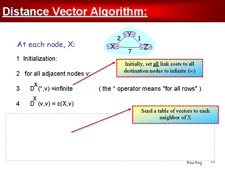
Distance Vector Algorithm: At each node, X: 1 Initialization: 2 for all adjacent nodes v: 3 4 X D (*, v) =infinite Y 7 1 Z Initially, set all link costs to all destination nodes to infinite (∞) ( the * operator means "for all rows" ) X D (v, v) = c(X, v) 5 for all destinations, y 6 X 2 Send a table of vectors to each neighbor of X X send min D (y, w) to each neighbor (w over all X's neighbors ) w Routing 13

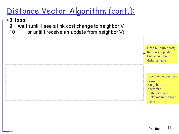
Distance Vector Algorithm (cont. ): 8 loop 9 wait (until I see a link cost change to neighbor V 10 or until I receive an update from neighbor V) 11 //link cost change 12 if (c(X, V) changes by d) 13 /* change cost to all dest's via neighbor v by d */ 14 /* note: d could be positive or negative */ 15 for all destinations y: DX(y, V) = DX(y, V) + d 16 //receipt of routing table from neighbor V 17 else if (update received from V wrt destination Y) Y 18 /* shortest path from V to some Y has changed */ 19 /* V has sent a new value for its min DV(Y, w) */ w 20 /* call this received new value as newval */ 21 for the single destination y: DX(Y, V) = c(X, V) + newval 22 //new least-cost to any destination Y found X 23 if we have a new min w D (Y, w) for any destination Y 24 send new value of min w DX(Y, w) to all neighbors 25 26 forever Change in link cost; therefore, update Entire column in distance table Received one update from neighbor v; therefore, Calculate new link cost in distance table Routing 14

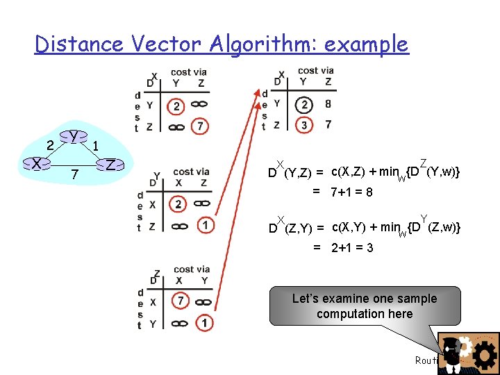
Distance Vector Algorithm: example X 2 Y 7 1 Z Z X D (Y, Z) = c(X, Z) + minw{D (Y, w)} = 7+1 = 8 Y X D (Z, Y) = c(X, Y) + minw {D (Z, w)} = 2+1 = 3 Let’s examine one sample computation here Routing 15

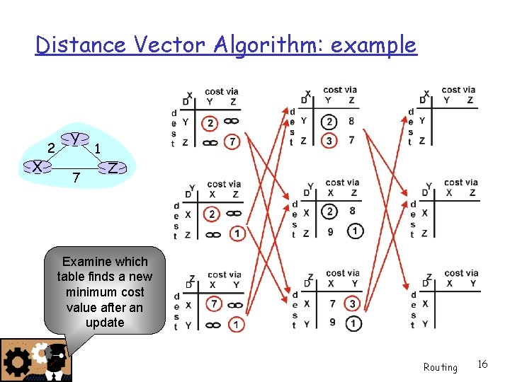
Distance Vector Algorithm: example X 2 Y 7 1 Z Examine which table finds a new minimum cost value after an update Routing 16

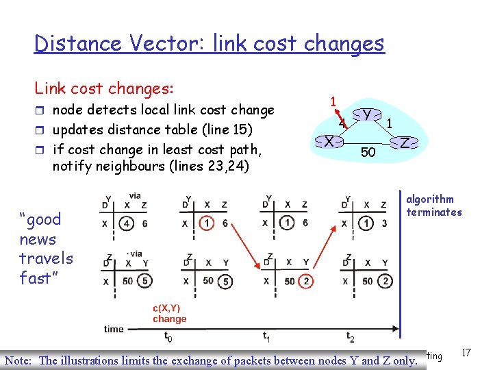
Distance Vector: link cost changes Link cost changes: node detects local link cost change updates distance table (line 15) if cost change in least cost path, notify neighbours (lines 23, 24) “good news travels fast” 1 4 X Y 50 1 Z algorithm terminates Routing Note: The illustrations limits the exchange of packets between nodes Y and Z only. 17

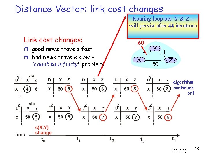
Distance Vector: link cost changes Routing loop bet. Y & Z – will persist after 44 iterations Link cost changes: good news travels fast bad news travels slow - 'count to infinity' problem! 60 4 X Y 50 1 Z algorithm continues on! Routing 18

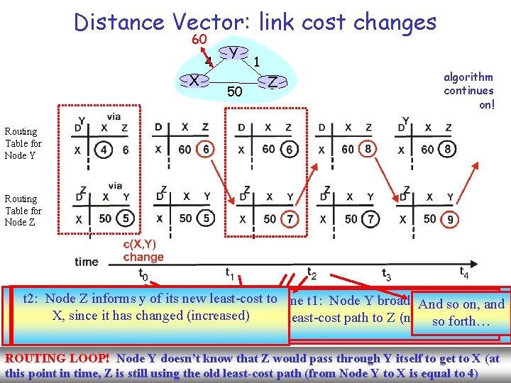
Distance Vector: link cost changes 60 4 X Y 50 1 Z algorithm continues on! Routing Table for Node Y Routing Table for Node Z after computes the new least-cost X, At t 2: Node Z informs y of new Sometime least-cost after tot 0: Y calculates the. And new least-cost Sometime t 1: Node Zits receives thetonew time. Node t 1: Node Y broadcasts the new so on, and Link-cost change: the new link-cost to X changes from then updates its Routing Table X, since it has changed (increased) path, and finds least-cost that passing through Z is so more cost least-cost to Node X from Y, then computes path to Z (neighbor) forth… to reach 60. Node X effective 4 to a new least-cost to X ROUTING LOOP! Node Y doesn’t know that Z would pass through Y itself to get to X (at 19 Routing this point in time, Z is still using the old least-cost path (from Node Y to X is equal to 4)

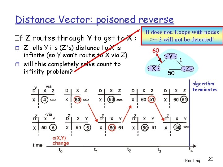
Distance Vector: poisoned reverse If Z routes through Y to get to X : Z tells Y its (Z's) distance to X is infinite (so Y won’t route to X via Z) will this completely solve count to infinity problem? It does not. Loops with nodes >= 3 will not be detected! 60 4 X Y 50 1 Z algorithm terminates Routing 20

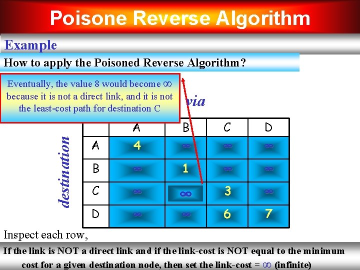
Poisone Reverse Algorithm Example How to apply the Poisoned Reverse Algorithm? destination Eventually, the value 8 would become ∞ because it is not a direct link, and it is not the least-cost path for destination C via A A 4 B ∞ C ∞ D ∞ B ∞ 1 ∞ ∞ C ∞ 8 ∞ 3 ∞ D ∞ ∞ 6 7 Inspect each row, If the link is NOT a direct link and if the link-cost is NOT equal to the minimum 21 Routing cost for a given destination node, then set the link-cost = ∞ (infinite)

Link-State Routing Algorithm Dijkstra’s algorithm • net topology, link costs known to all nodes – accomplished via “link state broadcast” – all nodes have the same info • computes least cost paths from one node (‘source”) to all other nodes – gives forwarding table for that node • iterative: after k iterations, know least cost path to k dest. ’s Notation: • c(x, y): link cost from node x to y; set equal to ∞ if not direct neighbors • D(v): current value of cost of path from source to dest. v • p(v): predecessor node along path from source to v • N': set of nodes whose least cost path definitively known 22

Dijsktra’s Algorithm 1 Initialization: 2 N' = {u} 3 for all nodes v 4 if v adjacent to u 5 then D(v) = c(u, v) 6 else D(v) = ∞ 7 8 Loop 9 find w not in N' such that D(w) is a minimum 10 add w to N' 11 update D(v) for all v adjacent to w and not in N' : 12 D(v) = min( D(v), D(w) + c(w, v) ) 13 /* new cost to v is either old cost to v or known 14 shortest path cost to w plus cost from w to v */ 15 until all nodes in N' 23

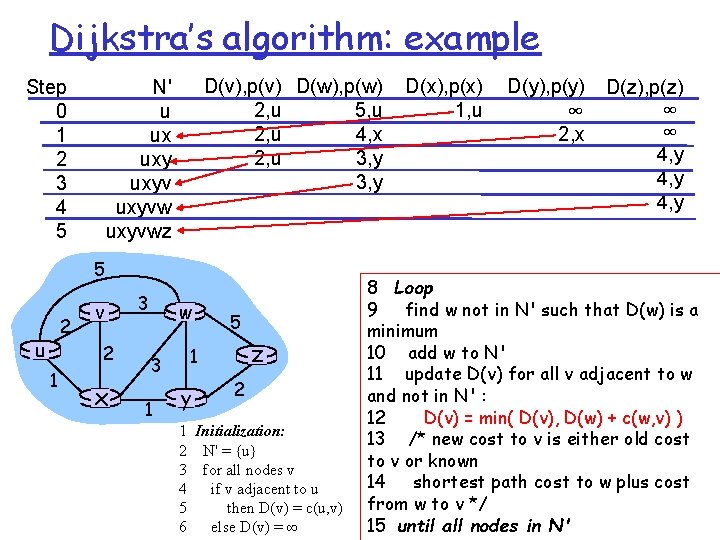
Dijkstra’s algorithm: example Step 0 1 2 3 4 5 D(v), p(v) D(w), p(w) 2, u 5, u 2, u 4, x 2, u 3, y N' u ux uxyvwz 5 2 u v 2 1 x 3 w 3 1 5 z 1 y 2 1 Initialization: 2 N' = {u} 3 for all nodes v 4 if v adjacent to u 5 then D(v) = c(u, v) 6 else D(v) = ∞ D(x), p(x) 1, u D(y), p(y) ∞ 2, x D(z), p(z) ∞ ∞ 4, y 8 Loop 9 find w not in N' such that D(w) is a minimum 10 add w to N' 11 update D(v) for all v adjacent to w and not in N' : 12 D(v) = min( D(v), D(w) + c(w, v) ) 13 /* new cost to v is either old cost to v or known 14 shortest path cost to w plus cost from w to v */ 24 15 until all nodes in N'

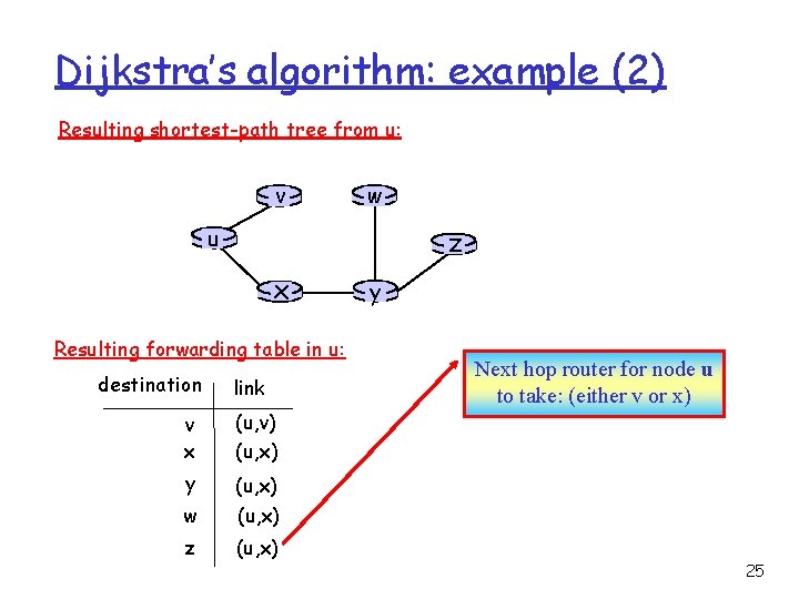
Dijkstra’s algorithm: example (2) Resulting shortest-path tree from u: v w u z x Resulting forwarding table in u: destination link v x (u, v) (u, x) y (u, x) w (u, x) z (u, x) y Next hop router for node u to take: (either v or x) 25

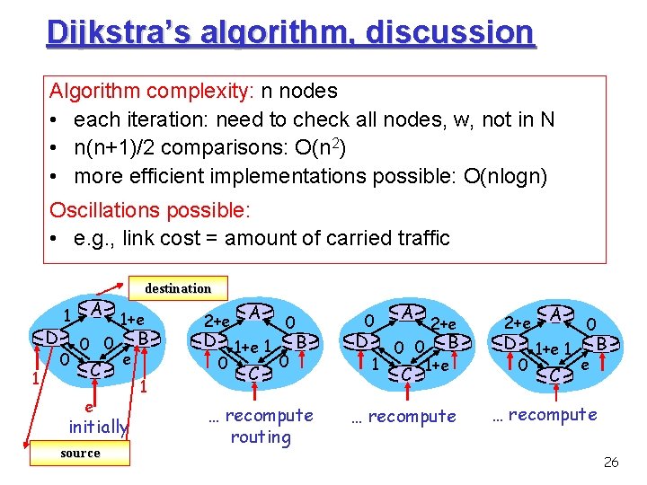
Dijkstra’s algorithm, discussion Algorithm complexity: n nodes • each iteration: need to check all nodes, w, not in N • n(n+1)/2 comparisons: O(n 2) • more efficient implementations possible: O(nlogn) Oscillations possible: • e. g. , link cost = amount of carried traffic D 1 1 0 A 0 0 C e destination 1+e e initially source B 1 2+e A 0 D 1+e 1 B 0 0 C … recompute routing 0 D 1 A 0 0 C 2+e B 1+e … recompute 2+e A 0 D 1+e 1 B e 0 C … recompute 26

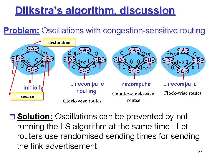
Dijkstra’s algorithm, discussion Problem: Oscillations with congestion-sensitive routing D 1 1 0 A 0 0 C e destination 1+e e initially source B 1 2+e A 0 D 1+e 1 B 0 0 C … recompute routing Clock-wise routes 0 D 1 A 0 0 C 2+e B 1+e … recompute Counter-clock-wise routes 2+e A 0 D 1+e 1 B e 0 C … recompute Clock-wise routes Solution: Oscillations can be prevented by not running the LS algorithm at the same time. Let routers use randomised sending times for sending the link advertisement. 27