Network Layer Design Issues Implementation of Connectionless Service

Network Layer Design Issues

§ Implementation of Connectionless Service § Implementation of Connection-Oriented Service § Comparison of Virtual-Circuit and Datagram Subnets

Main objective • Data delivery from source to destination

Connectionless services

Connectionless-Oriented services • Logical connection is established

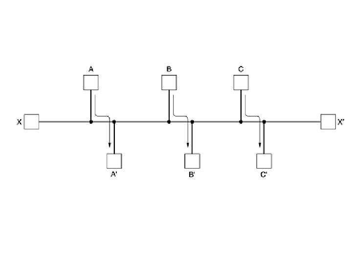
Implementation of Connectionless Service Routing within a datagram subnet. (destined for, outgoing line)

Datagram: • With a datagram, the router from source to destination are not worked out in advance. • Each packet sent is routed independently. • Successive packets can follow different routes. • The datagram subnet have to do more work but they are more robust and deal with failures and congestion.

Implementation of Connection-Oriented Service Routing within a VC subnet (incoming, connection id) (outgoing, connection id)

Virtual Circuits: • The principal behind the virtual circuits is to choose only one route from source to destination. • When a connection is established, it is used for all the traffic flowing over the connection. • When the connection is released , the virtual circuits is terminated.

Issue Datagram Subnet VC Subnet Connection-less service Connection-Oriented Service Circuit set up Not required Required Addressing Each packet contains a the source as well as short VC number. Only the first packets contain destination address the source and destination address to set up the connection. State information Subnet does not hold state information A table is needed to hold the state information Routing Each packet is routed independently Route chosen when VC is setup; all packet follow this route Congestion control Easy if enough Difficult resources can be allocated in advance for each VC.

Issue Datagram Subnet VC Subnet Quality of service Easy if enough Difficult resources can be allocated in advance for each VC. Effect of router failure No other effect except for the packets lost at the time of crash All VCs which passed through failed router are terminated. Path No dedicated path, each follows its own path All packets of the message follows same path Unit of data transmitted Packet Delay Packet transmission delay only Connection setup and transmission delay Overload Each Packet contain header Only setup packets contain header

Issue Datagram Subnet VC Subnet Resource Reservation Resources are not reserved Resources are reserved during setup phase only and maintained until the data transfer phase Upper layer Protocol used UDP over IP TCP over IP Vulnerability Less Vulnerable, More Robust Vulnerable

Routing Algorithms • Routing Algorithm: is that part of the network layer software responsible for deciding which output line an incoming packet should be transmitted on

• Routing Algorithm for Datagram always anew • Routing algorithm for Virtual Circuit remains same for user session : Session Routing • Role of Router: – Forwarding – Updating routing table • Forwarding: Making the decision which routes to use when a packet arrives. - handles each packet as it arrives, looking up the outgoing line to use for it in the routing tables. • Updating routing tables: responsible for filling in and updating the routing tables and the routing algorithm comes into play.

• Desirable Properties of a routing algorithm: correctness simplicity robustness stability fairness optimality

• Robustness: The routing algorithm should be able to cope with changes in the topology and traffic without requiring all jobs in all hosts to be aborted and the network to be rebooted every time some router crashes. • Stability : Routing algorithms reaches equilibrium and stays there. • Fairness & Optimality looks similar, but may be contradictory.

• Minimizing mean packet delay and maximizing total network throughput are rquired , but these two goals are also in conflict. • Since operating any queueing system near capacity implies a long queueing delay. • As a compromise, many networks attempt to minimize the number of hops a packet must make, because reducing the number of hops tends to improve the delay and also reduce the amount of bandwidth consumed, which tends to improve throughput as well.

• Routing algorithms - two major classes: nonadaptive. • Nonadaptive algorithms The choice of the route to use from I to J (for all I and J) is computed in advance, off-line, and downloaded to the routers when the network is booted. Aslo called static routing.

• Adaptive algorithms Change their routing decisions to reflect changes in the topology, and usually the traffic as well. Aslo called dynamic routing • Adaptive algorithms differ in • where they get their information (e. g. , locally, from adjacent routers, or from all routers), • when they change the routes (e. g. , every ΔT sec, when the load changes or when the topology changes), • what metric is used for optimization (e. g. , distance, number of hops, or estimated transit time).

The Optimality Principle • optimality principle states that if router J is on the optimal path from router I to router K, then the optimal path from J to K also falls along the same route. • Say the part of the route from I to J is r 1 and the rest of the route r 2. If a route better than r 2 existed from J to K, it could be concatenated with r 1 to improve the route from I to K, contradicting our statement that r 1 r 2 is optimal.

Sink Tree

Sink Tree • A direct consequence of the optimality principle, is the set of optimal routes from all sources to a given destination form a tree rooted at the destination. Such a tree is called a sink tree • Here the distance metric is the number of hops. • The goal of all routing algorithms is to discover and use the sink trees for all routers.

Sink Tree • Sink tree is not necessarily unique; other trees with the same path lengths may exist. • No loops • Each packet is made sure to be delivered within finite no. of hops.

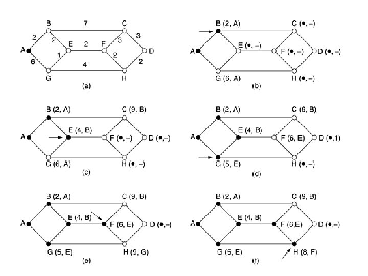
Shortest Path Routing • Graph of the subnet: each node- a router each arc-communication line • Shortest path routing algorithm chooses a shortest possible route between a given pair of routers.

• Label on arc is computed as a function of: – distance – Bandwidth – average traffic – communication cost – mean queue length – measured delay – and other factors, etc. • This is also called as weight of the edge / link.

• Many shortest path Algorithms, but Dijkstra is most widely studied.

FLOODING • Flooding - static algorithm, every incoming packet is sent out on every outgoing line except the one it arrived on. • Generates vast numbers of duplicate packets. • Hop counter in header of each packet is included and is decremented at each hop to reduce duplicates. • Packet is discarded when the counter reaches zero.

FLOODING • Hop counter is set to the length of the path from source to destination, if length is known, else given the logest path length of subnet. • An alternative technique for damming the flood is to keep track of which packets have been • flooded, to avoid sending them out a second time. achieve this goal is to have the source • router put a sequence number in each packet it receives from its hosts. Each router then • needs a list per source router telling which

selective flooding • Routers do not send every incoming packet out on every line, only on those lines that are going approximately in the right direction. • Eg: There is usually little point in sending a westbound packet on an eastbound line.

• Flooding is not practical in most applications, but has some uses. • For example, in military applications, where large numbers of routers may be blown to bits at any instant, the tremendous robustness of flooding is highly desirable. • In distributed database applications, it is sometimes necessary to update all the databases concurrently, in which case flooding can be useful.

• In wireless networks, all messages transmitted by a station can be received by all other stations within its radio range, which is, in fact, flooding. • Used as a metric against which other routing algorithms can be compared. • Flooding always chooses the shortest path because it chooses every possible path in parallel.

Broadcast Routing • Used when hosts need to send messages to many or all other hosts. • Egs: a service distributing weather reports, stock market updates, or live radio programs, etc • Sending a packet to all destinations simultaneously is called broadcasting • Various methods have been proposed for this.

Broadcast Routing • One broadcasting method: requires no special features from the subnet is for the source to simply send a distinct packet to each destination. • Here the disadvantage – wastes the bandwidth - requires the source to have a complete list of all destinations.

• Flooding is another opion, but it carries its own disadvantages. It generates too many packets and consumes too much bandwidth. • A third algorithm is multidestination routing. • Here each packet contains either a list of destinations or a bit map indicating the desired destinations. • When a packet arrives at a router, the router checks all the destinations to determine the set of output lines that will be needed. (An output line is needed if it is the best route to at least one of the destinations. )

• The router generates a new copy of the packet for each output line to be used and includes in each packet only those destinations that are to use the line. • In effect, the destination set is partitioned among the output lines. After a sufficient number of hops, each packet will carry only one destination and can be treated as a normal packet.

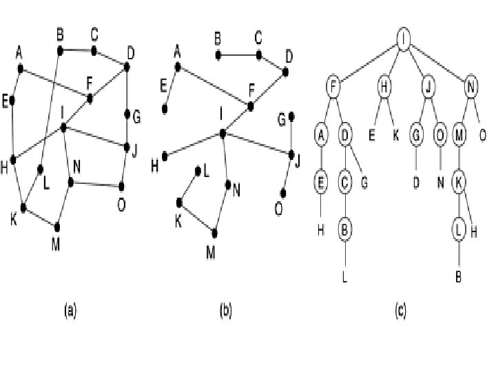
• A fourth broadcast algorithm uses the sink tree for the router initiating the broadcast—or any other convenient spanning tree for that matter. • If each router knows which of its lines belong to the spanning tree, it can copy an incoming broadcast packet onto all the spanning tree lines except the one it arrived on and generating the absolute minimum number of packets and efficiet use of badwidth. • Main hurdle is each router must have knowledge of some spanning tree, which depends on the inner algorithm followed.

• To overcome the knowledge of spanning tree, reverse path forwarding, is used. • When a broadcast packet arrives at a router, the router checks to see if the packet arrived on the line that is normally used for sending packets to the source of the broadcast. • If so, there is an excellent chance that the broadcast packet itself followed the best route from the router and is therefore the first copy to arrive at the router. This being the case, the router forwards copies of it onto all lines except the one it arrived on. If, however, the broadcast packet arrived on a line other than the preferred one for reaching the source, the packet is discarded as a likely duplicate.

• Principal advantage - reasonably efficient and easy to implement. • No overhead of a destination list or bit map in each broadcast packet as does multidestination addressing. • Doesn’t require any special mechanism to stop the process like flooding.

Multicast Routing • Some applications require that widelyseparated processes work together in groups, for example, a group of processes implementing a distributed database system. • In these situations, it is frequently necessary for one process to send a message to all the other members of the group. • If the group is small, it can just send each other member a point-to-point message.

• If the group is large, this strategy is expensive. • Sometimes broadcasting can be used, but using broadcasting to inform 1000 machines on a million-node network is inefficient. • Sending a message to well-defined groups that are numerically large in size but small compared to the network as a whole is called multicasting, and its routing algorithm is called multicast routing.

• Multicasting requires group management – acts like creation and destruction of groups, allow processes to join and leave groups routing algorithm is not conerned about these actions. • Routing algorithm is responsible that when a process joins a group, it informs its host of this fact.

• It is important that routers know which of their hosts belong to which groups. Either hosts must inform their routers about changes in group membership, or routers must query their hosts periodically. Either way, routers learn about which of their hosts are in which groups. • Routers tell their neighbors, so the information propagates through the subnet.

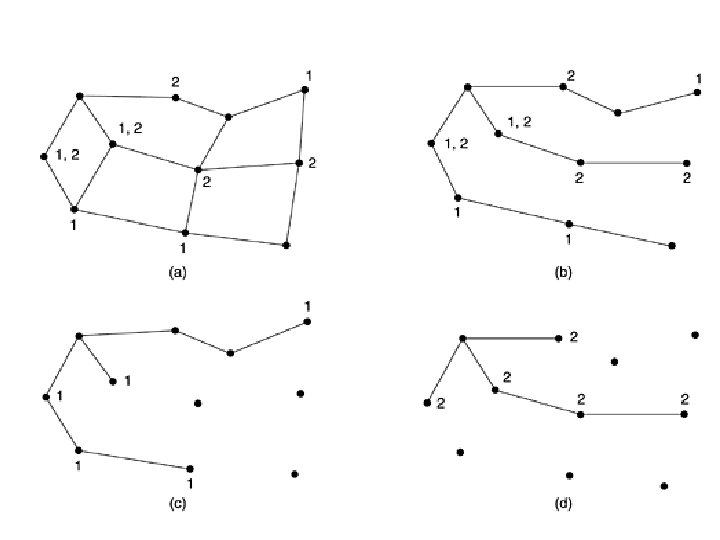
• To do multicast routing, each router computes a spanning tree covering all other routers. • For example, in Fig. 5 -17(a) we have two groups, 1 and 2. Some routers are attached to hosts that belong to one or both of these groups, as indicated in the figure. A spanning tree for the leftmost router is shown in Fig. 517(b).

• When a process sends a multicast packet to a group, the first router examines its spanning tree and prunes it, removing all lines that do not lead to hosts that are members of the group. • In our example, Fig. 5 -17(c) shows the pruned spanning tree for group 1. Similarly, Fig. 517(d) shows the pruned spanning tree for group 2.

• Various ways of pruning the spanning tree are possible. – Link State Routing – Distance Vector Routing • Disadvantage – high no. in network leads to poor working – Design using core-based trees

Distance Vector Routing • Two most popular dynamic algorithms used in modern networks in particular are, distance vector routing and link state routing. • The distance vector also known as distributed Bellman-Ford routing algorithm and the Ford. Fulkerson algorithm. • It was the original ARPANET routing algorithm and was also used in the Internet under the name RIP.

• Distance vector routing algorithms operate by having each router maintain a routing table (vector) indexed by, and containing one entry for, each router in the subnet, giving the best known distance to each destination and which line to use to get there. • These tables are updated by exchanging information with the neighbors.

• The entry in the table contains two parts: the preferred outgoing line to use for that destination and an estimate of the time or distance to that destination. • The router is assumed to know the ''distance'' to each of its neighbors. • The metric used might be – number of hops – time delay in milliseconds - router measures it directly with special ECHO packets that the receiver just timestamps and sends back as fast as it can. – total number of packets queued along the path - the router examines each queue – etc.

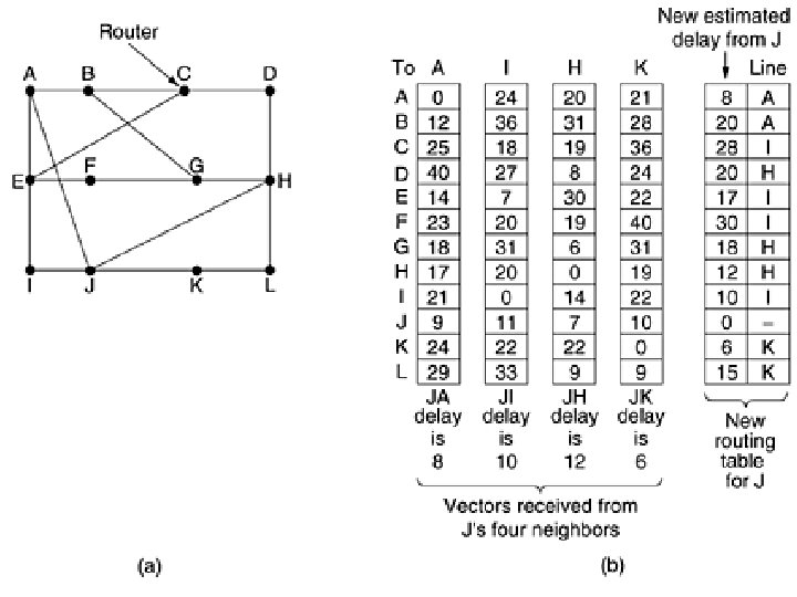
• Example - delay is used as a metric and that the router knows the delay to each of its neighbors. • Once every T msec each router sends to each neighbor a list of its estimated delays to each destination. • It also receives a similar list from each neighbor. • Say tables has just come in from neighbor X, with XI(X-I) is esstimate to reach router I from X • If the router knows that the delay to X is m msec, it also knows that it can reach router I via X in XI + m msec.

• Similar calculations applied to estimate the best and use the corresponding line in its new routing table. Note that the old routing table is not used in the calculation. • This updating process is illustrated in Fig. 5 -9. Part (a) shows a subnet. The first four columns of part (b) show the delay vectors received from the neighbors of router J. A claims to have a 12 -msec delay to B, a 25 -msec delay to C, a 40 -msec delay to D, etc. Suppose that J has measured or estimated its delay to its neighbors, A, I, H, and K as 8, 10, 12, and 6 msec, respectively.

• Consider how J computes its new route to router G. It knows that it can get to A in 8 msec, and A claims to be able to get to G in 18 msec, so J knows it can count on a delay of 26 msec to G if it forwards packets bound for G to A. • Similarly, it computes the delay to G via I, H, and K as 41 (31 + 10), 18 (6 + 12), and 37 (31 + 6) msec, respectively. • The best of these values is 18, so it makes an entry in its routing table that the delay to G is 18 msec and that the route to use is via H.

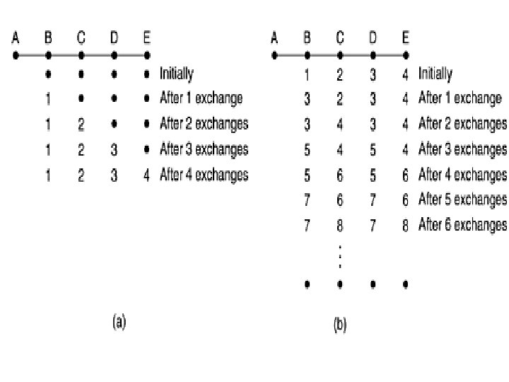
The Count-to-Infinity Problem • Distance vector drawback, practical implementation • Though it converges to the correct answer, it may do so slowly. • Reacts rapidly to good news, but leisurely to bad news. • Consider a router whose best route to destination X is large. • If on the next exchange neighbor A suddenly reports a short delay to X, the router just switches over to using the line to A to send traffic to X. • In one vector exchange, the good news is processed.

• No router ever has a value more than one higher than the minimum of all its neighbors. • Gradually, all routers work their way up to infinity, but involves considerably large no. of exchanges. It is wise to set infinity to the longest path plus 1. • If the metric is time delay, there is no well-defined upper bound, so a high value is needed to prevent a path with a long delay from being treated as down. • This problem is known as the count-to-infinity problem.

• Few solutions are – Split horizon with poisoned reverse - but none of these work well in general. • The problem is that when X tells Y that it has a path somewhere, Y has no way of knowing whether it itself is on the path.

Hierarchical Routing • As networks grow in size, the router routing tables grow proportionally. • Not only is router memory consumed by everincreasing tables, but more CPU time is needed to scan them and more bandwidth is needed to send status reports about them. • At a certain point the network may grow to the point where it is no longer feasible for every router to have an entry for every other router, so the routing will have to be done hierarchically, as it is in the telephone network.

Hierarchical Routing • When hierarchical routing is used, the routers are divided into regions, with each router knowing all the details about how to route packets to destinations within its own region, but knowing nothing about the internal structure of other regions. • When different networks are interconnected, it is natural to regard each one as a separate region in order to free the routers in one network from having to know the topological structure of the other ones.

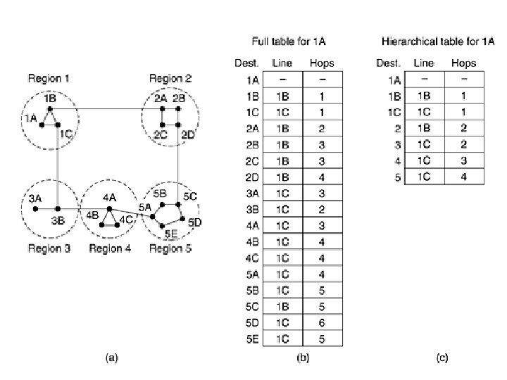
Hierarchical Routing • For huge networks, a two-level hierarchy may be insufficient; • It is necessary to group further like – the regions into clusters – the clusters into zones – the zones into groups and so on • Eg : consider a packet from Berkeley, California, to Malindi, Kenya.

• The Berkeley router would know the detailed topology within California but would send all out-ofstate traffic to the Los Angeles router. • The Los Angeles router would be able to route traffic to other domestic routers but would send foreign traffic to New York. • The New York router would be programmed to direct all traffic to the router in the destination country responsible for handling foreign traffic, say, in Nairobi. Finally, the packet would work its way down the tree in Kenya until it got to Malindi.

Pros & Cons of Hierarchical Routing • Advantage is gain in pain and computation. • Disadvantage – is increased path length. – For example, the best route from 1 A to 5 C is via region 2, but with hierarchical routing all traffic to region 5 goes via region 3, because that is better for most destinations in region 5.

Optimial No. of Levels in Hierarchy • How many levels should the hierarchy have & How many groups in each hierarchy. – For example: consider a subnet with 720 routers. – If there is no hierarchy : each router needs 720 routing table entries. – If the subnet is partitioned into 24 regions of 30 routers each, each router needs 30 local entries plus 23 remote entries for a total of 53 entries.

Optimial No. of Levels in Hierarchy – If a three-level hierarchy is chosen, with eight clusters, each containing 9 regions of 10 routers, each router needs 10 entries for local routers, 8 entries for routing to other regions within its own cluster, and 7 entries for distant clusters, for a total of 25 entries. • Kamoun and Kleinrock (1979) discovered that the optimal number of levels for an N router subnet is ln. N, requiring a total of eln. N entries per router and provides an effective path length