Network Layer Control Plane COMPSCI 453 Computer Networks

Network Layer: Control Plane COMPSCI 453 Computer Networks Professor Jim Kurose College of Information and Computer Sciences University of Massachusetts § introduction § routing algorithms § link state § distance vector § intra-ISP routing: OSPF § routing among ISPs: BGP § SDN control plane § Internet Control Message Protocol § Network management, configuration Class textbook: Computer Networking: A Top. Down Approach (8 th ed. ) J. F. Kurose, K. W. Ross Pearson, 2020 http: //gaia. cs. umass. edu/kurose_ross

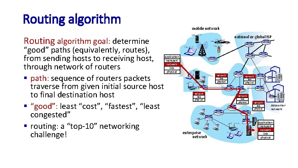
Routing algorithm mobile network national or global ISP Routing algorithm goal: determine “good” paths (equivalently, routes), from sending hosts to receiving host, through network of routers § path: sequence of routers packets traverse from given initial source host to final destination host § “good”: least “cost”, “fastest”, “least congested” § routing: a “top-10” networking challenge! application transport network link physical enterprise network link physical datacenter network application transport network link physical

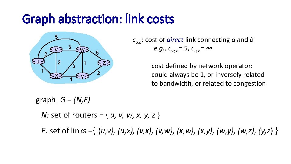
Graph abstraction: link costs 5 2 u v 2 1 x 3 w 3 1 5 z 1 y ca, b: cost of direct link connecting a and b e. g. , cw, z = 5, cu, z = ∞ 2 cost defined by network operator: could always be 1, or inversely related to bandwidth, or related to congestion graph: G = (N, E) N: set of routers = { u, v, w, x, y, z } E: set of links ={ (u, v), (u, x), (v, w), (x, y), (w, z), (y, z) }

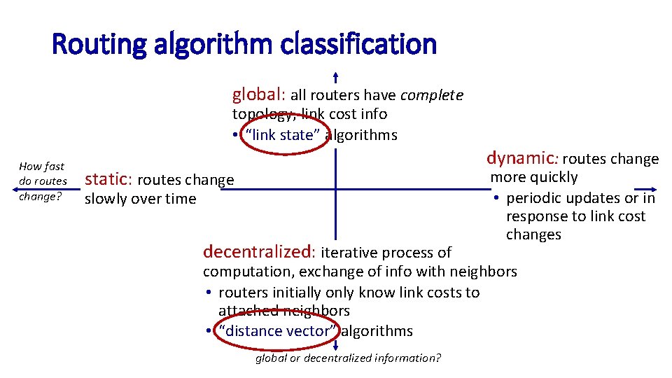
Routing algorithm classification global: all routers have complete topology, link cost info • “link state” algorithms How fast do routes change? dynamic: routes change static: routes change slowly over time decentralized: iterative process of more quickly • periodic updates or in response to link cost changes computation, exchange of info with neighbors • routers initially only know link costs to attached neighbors • “distance vector” algorithms global or decentralized information?

Network layer: “control plane” roadmap § introduction § routing protocols § link state § distance vector § intra-ISP routing: OSPF § routing among ISPs: BGP § SDN control plane § Internet Control Message Protocol § network management, configuration • SNMP • NETCONF/YANG

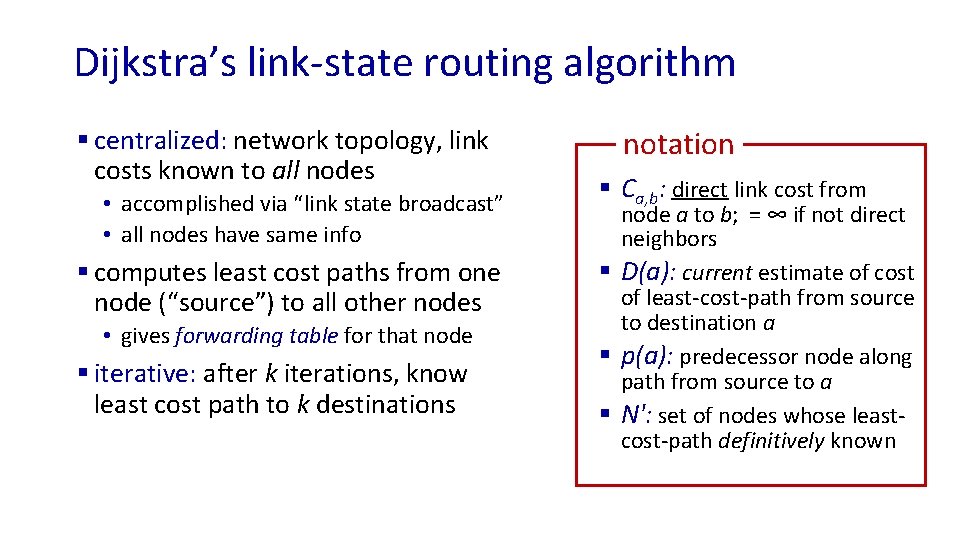
Dijkstra’s link-state routing algorithm § centralized: network topology, link costs known to all nodes • accomplished via “link state broadcast” • all nodes have same info § computes least cost paths from one node (“source”) to all other nodes • gives forwarding table for that node § iterative: after k iterations, know least cost path to k destinations notation § Ca, b: direct link cost from node a to b; = ∞ if not direct neighbors § D(a): current estimate of cost of least-cost-path from source to destination a § p(a): predecessor node along path from source to a § N': set of nodes whose leastcost-path definitively known

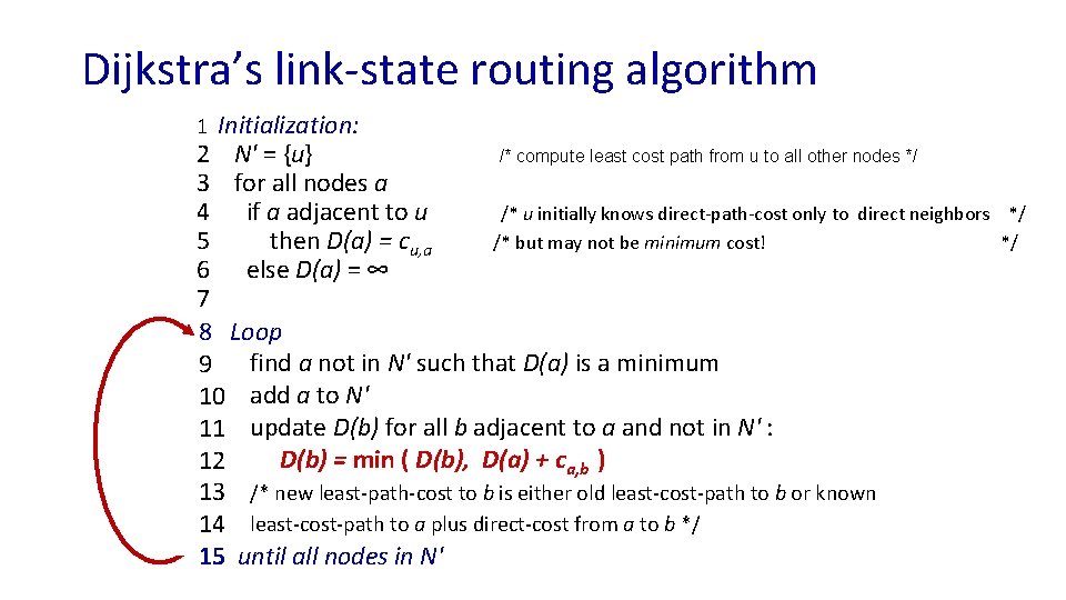
Dijkstra’s link-state routing algorithm Initialization: 2 N' = {u} /* compute least cost path from u to all other nodes */ 3 for all nodes a 4 if a adjacent to u /* u initially knows direct-path-cost only to direct neighbors 5 then D(a) = cu, a /* but may not be minimum cost! 6 else D(a) = ∞ 7 8 Loop 9 find a not in N' such that D(a) is a minimum 10 add a to N' 11 update D(b) for all b adjacent to a and not in N' : D(b) = min ( D(b), D(a) + ca, b ) 12 13 /* new least-path-cost to b is either old least-cost-path to b or known 14 least-cost-path to a plus direct-cost from a to b */ 15 until all nodes in N' 1 */ */

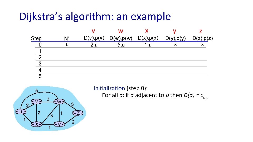
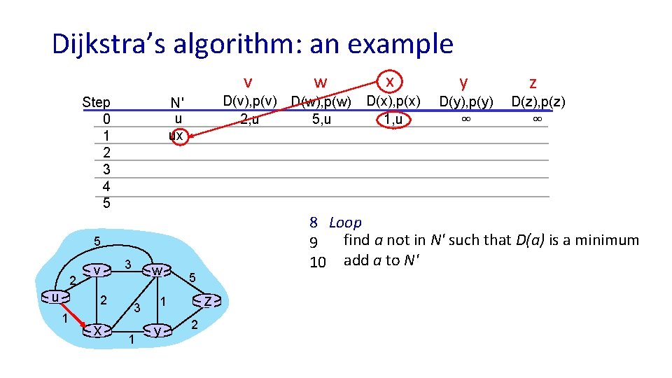
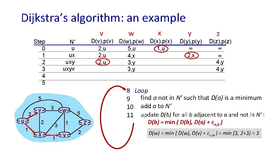
Dijkstra’s algorithm: an example v Step 0 1 2 3 4 5 D(v), p(v) D(w), p(w) 5, u 2, u N' u 2 1 x 3 w 3 1 5 z 1 y x y D(x), p(x) 1, u D(y), p(y) D(z), p(z) ∞ ∞ z Initialization (step 0): For all a: if a adjacent to u then D(a) = cu, a 5 v w 2

Dijkstra’s algorithm: an example v Step 0 1 2 3 4 5 D(v), p(v) D(w), p(w) 5, u 2, u N' u ux 2 u 2 1 x 3 w 3 1 5 z 1 y 2 x y D(x), p(x) 1, u D(y), p(y) D(z), p(z) ∞ ∞ z 8 Loop find a not in N' such that D(a) is a minimum 9 10 add a to N' 5 v w

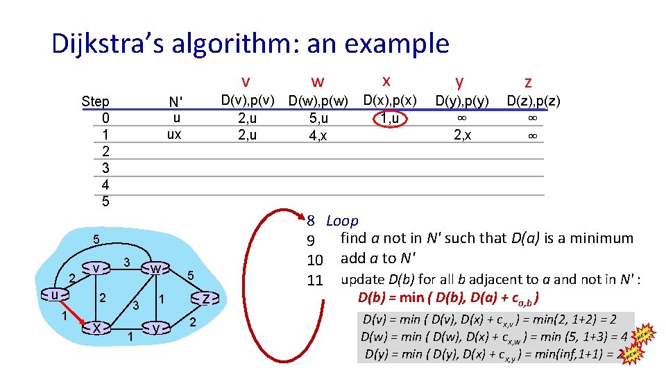
Dijkstra’s algorithm: an example v Step 0 1 2 3 4 5 D(v), p(v) D(w), p(w) 5, u 2, u 4, x N' u ux 5 2 u v 2 1 x 3 w 3 1 5 z 1 y w 2 x y D(x), p(x) 1, u D(y), p(y) D(z), p(z) ∞ ∞ ∞ 2, x z 8 Loop find a not in N' such that D(a) is a minimum 9 10 add a to N' 11 update D(b) for all b adjacent to a and not in N' : D(b) = min ( D(b), D(a) + ca, b ) D(v) = min ( D(v), D(x) + cx, v ) = min(2, 1+2) = 2 D(w) = min ( D(w), D(x) + cx, w ) = min (5, 1+3) = 4 D(y) = min ( D(y), D(x) + cx, y ) = min(inf, 1+1) = 2

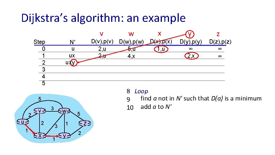
Dijkstra’s algorithm: an example v Step 0 1 2 3 4 5 D(v), p(v) D(w), p(w) 5, u 2, u 4, x N' u ux uxy 2 u 2 1 x 3 w 3 1 5 z 1 y 2 x y D(x), p(x) 1, u D(y), p(y) D(z), p(z) ∞ ∞ ∞ 2, x z 8 Loop find a not in N' such that D(a) is a minimum 9 10 add a to N' 5 v w

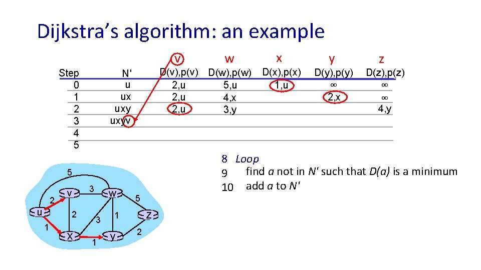
Dijkstra’s algorithm: an example v Step 0 1 2 3 4 5 D(v), p(v) D(w), p(w) 5, u 2, u 4, x 2, u 3, y N' u ux uxy 5 2 u v 2 1 x 3 w 3 1 5 z 1 y w 2 x y D(x), p(x) 1, u D(y), p(y) D(z), p(z) ∞ ∞ ∞ 2, x z 4, y 8 Loop find a not in N' such that D(a) is a minimum 9 10 add a to N' 11 update D(b) for all b adjacent to a and not in N' : D(b) = min ( D(b), D(a) + ca, b ) D(w) = min ( D(w), D(y) + cx, w ) = min (4, 2+1) = 3 D(z) = min ( D(z), D(y) + cy, x ) = min(inf, 2+2) = 4

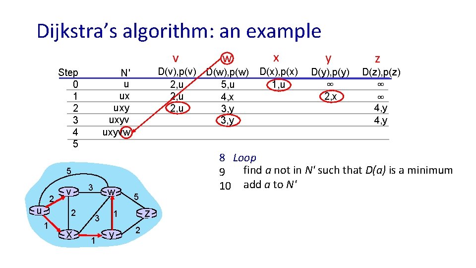
Dijkstra’s algorithm: an example v Step 0 1 2 3 4 5 D(v), p(v) D(w), p(w) 5, u 2, u 4, x 2, u 3, y N' u ux uxyv 2 u 2 1 x 3 w 3 1 5 z 1 y 2 x y D(x), p(x) 1, u D(y), p(y) D(z), p(z) ∞ ∞ ∞ 2, x z 4, y 8 Loop find a not in N' such that D(a) is a minimum 9 10 add a to N' 5 v w

Dijkstra’s algorithm: an example v Step 0 1 2 3 4 5 D(v), p(v) D(w), p(w) 5, u 2, u 4, x 2, u 3, y N' u ux uxyv 5 2 u v 2 1 x 3 w 3 1 5 z 1 y w 2 x y D(x), p(x) 1, u D(y), p(y) D(z), p(z) ∞ ∞ ∞ 2, x z 4, y 8 Loop find a not in N' such that D(a) is a minimum 9 10 add a to N' 11 update D(b) for all b adjacent to a and not in N' : D(b) = min ( D(b), D(a) + ca, b ) D(w) = min ( D(w), D(v) + cv, w ) = min (3, 2+3) = 3

Dijkstra’s algorithm: an example v Step 0 1 2 3 4 5 D(v), p(v) D(w), p(w) 5, u 2, u 4, x 2, u 3, y N' u ux uxyvw 2 u 2 1 x 3 w 3 1 5 z 1 y 2 x y D(x), p(x) 1, u D(y), p(y) D(z), p(z) ∞ ∞ ∞ 2, x z 4, y 8 Loop find a not in N' such that D(a) is a minimum 9 10 add a to N' 5 v w

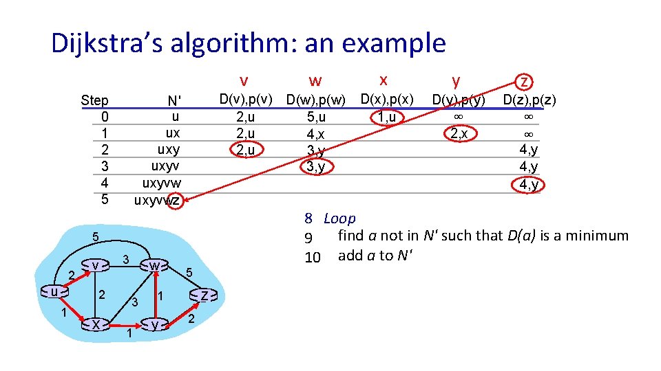
Dijkstra’s algorithm: an example v Step 0 1 2 3 4 5 D(v), p(v) D(w), p(w) 5, u 2, u 4, x 2, u 3, y N' u ux uxyvw 5 2 u v 2 1 x 3 w 3 1 5 z 1 y w 2 x y D(x), p(x) 1, u D(y), p(y) D(z), p(z) ∞ ∞ ∞ 2, x z 4, y 8 Loop find a not in N' such that D(a) is a minimum 9 10 add a to N' 11 update D(b) for all b adjacent to a and not in N' : D(b) = min ( D(b), D(a) + ca, b ) D(z) = min ( D(z), D(w) + cw, z ) = min (4, 3+5) = 4

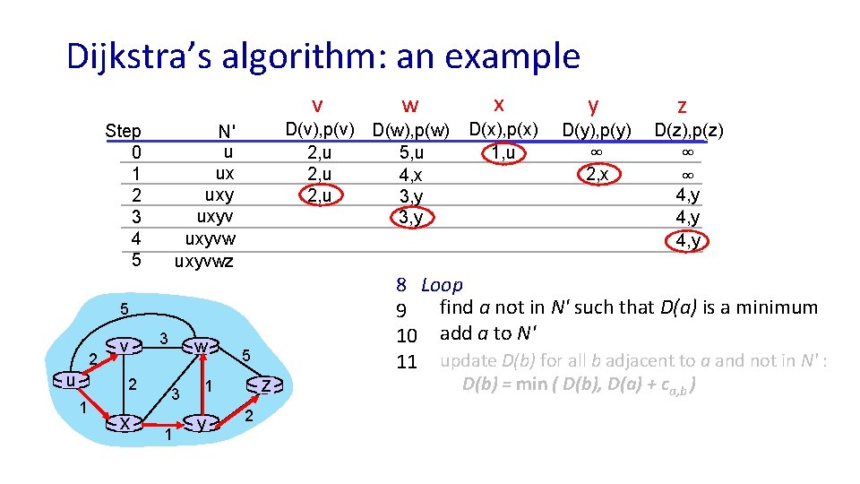
Dijkstra’s algorithm: an example v Step 0 1 2 3 4 5 D(v), p(v) D(w), p(w) 5, u 2, u 4, x 2, u 3, y N' u ux uxyvwz 2 u 2 1 x 3 w 3 1 5 z 1 y 2 x y D(x), p(x) 1, u D(y), p(y) D(z), p(z) ∞ ∞ ∞ 2, x z 4, y 8 Loop find a not in N' such that D(a) is a minimum 9 10 add a to N' 5 v w

Dijkstra’s algorithm: an example v Step 0 1 2 3 4 5 D(v), p(v) D(w), p(w) 5, u 2, u 4, x 2, u 3, y N' u ux uxyvwz 5 2 u v 2 1 x 3 w 3 1 5 z 1 y w 2 x y D(x), p(x) 1, u D(y), p(y) D(z), p(z) ∞ ∞ ∞ 2, x z 4, y 8 Loop find a not in N' such that D(a) is a minimum 9 10 add a to N' 11 update D(b) for all b adjacent to a and not in N' : D(b) = min ( D(b), D(a) + ca, b )

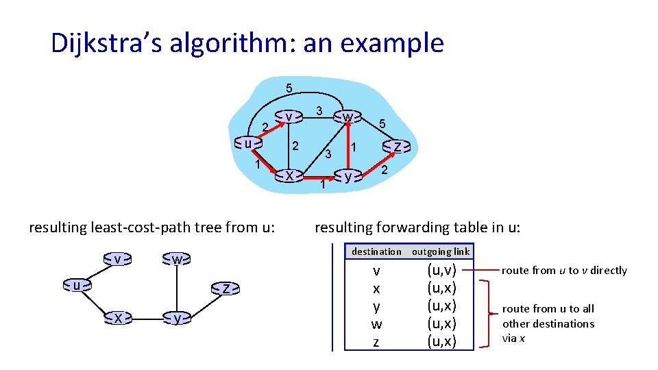
Dijkstra’s algorithm: an example 5 2 u 2 1 resulting least-cost-path tree from u: v z x y x 3 w 3 1 5 z 1 y 2 resulting forwarding table in u: destination outgoing link w u v v x y w z (u, v) (u, x) route from u to v directly route from u to all other destinations via x

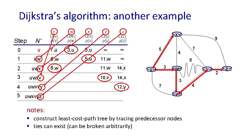
Dijkstra’s algorithm: another example v Step N' D(v), p(v) 0 u 7, u 1 uw 6, w 2 uwx 6, w 3 uwxv 4 uwxvy 5 uwxvyz w x y z D(w), p(w) D(x), p(x) D(y), p(y) D(z), p(z) 3, u 5, u ∞ ∞ 5, u 11, w ∞ 11, w 14, x 10, v 14, x 12, y x 5 9 7 4 8 3 u w y 3 7 v notes: § construct least-cost-path tree by tracing predecessor nodes § ties can exist (can be broken arbitrarily) 4 2 z

Dijkstra’s algorithm: discussion algorithm complexity: n nodes § each of n iteration: need to check all nodes, w, not in N § n(n+1)/2 comparisons: O(n 2) complexity § more efficient implementations possible: O(nlogn) message complexity: § each router must broadcast its link state information to other n routers § efficient (and interesting!) broadcast algorithms: O(n) link crossings to disseminate a broadcast message from one source § each router’s message crosses O(n) links: overall message complexity: O(n 2)

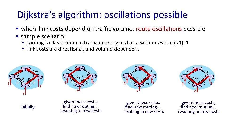
Dijkstra’s algorithm: oscillations possible § when link costs depend on traffic volume, route oscillations possible § sample scenario: • routing to destination a, traffic entering at d, c, e with rates 1, e (<1), 1 • link costs are directional, and volume-dependent a 1 d 1 0 0 0 c 2+e 1+e d b e e initially 1 1 a 0 c d b 1+e 1 0 0 0 1 e given these costs, find new routing…. resulting in new costs 1 a 0 1 c 2+e b 0 1+e 1 e given these costs, find new routing…. resulting in new costs d 1 a 0 b 1+e 1 0 c 0 1 e given these costs, find new routing…. resulting in new costs

Network Layer: Control Plane COMPSCI 453 Computer Networks Professor Jim Kurose College of Information and Computer Sciences University of Massachusetts § introduction § routing algorithms § link state § distance vector § intra-ISP routing: OSPF § routing among ISPs: BGP § SDN control plane § Internet Control Message Protocol § Network management, configuration Class textbook: Computer Networking: A Top. Down Approach (8 th ed. ) J. F. Kurose, K. W. Ross Pearson, 2020 http: //gaia. cs. umass. edu/kurose_ross

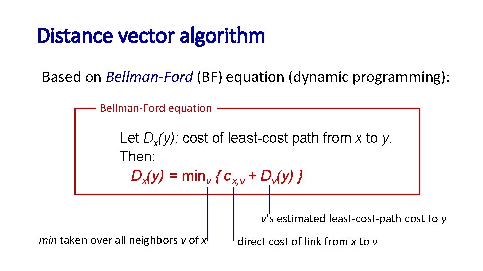
Distance vector algorithm Based on Bellman-Ford (BF) equation (dynamic programming): Bellman-Ford equation Let Dx(y): cost of least-cost path from x to y. Then: Dx(y) = minv { cx, v + Dv(y) } v’s estimated least-cost-path cost to y min taken over all neighbors v of x direct cost of link from x to v

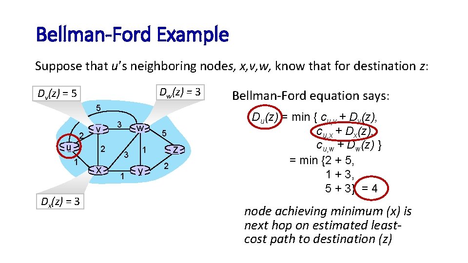
Bellman-Ford Example Suppose that u’s neighboring nodes, x, v, w, know that for destination z: Dw(z) = 3 Dv(z) = 5 5 2 u v 2 1 Dx(z) = 3 x 3 w 3 1 5 z 1 y 2 Bellman-Ford equation says: Du(z) = min { cu, v + Dv(z), cu, x + Dx(z), cu, w + Dw(z) } = min {2 + 5, 1 + 3, 5 + 3} = 4 node achieving minimum (x) is next hop on estimated leastcost path to destination (z)

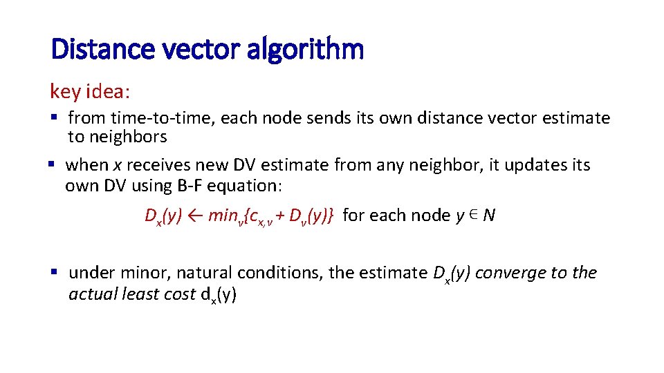
Distance vector algorithm key idea: § from time-to-time, each node sends its own distance vector estimate to neighbors § when x receives new DV estimate from any neighbor, it updates its own DV using B-F equation: Dx(y) ← minv{cx, v + Dv(y)} for each node y ∊ N § under minor, natural conditions, the estimate Dx(y) converge to the actual least cost dx(y)

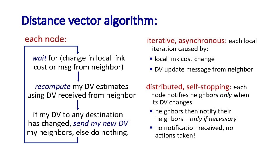
Distance vector algorithm: each node: wait for (change in local link cost or msg from neighbor) recompute my DV estimates using DV received from neighbor if my DV to any destination has changed, send my new DV my neighbors, else do nothing. iterative, asynchronous: each local iteration caused by: § local link cost change § DV update message from neighbor distributed, self-stopping: each node notifies neighbors only when its DV changes § neighbors then notify their neighbors – only if necessary § no notification received, no actions taken!

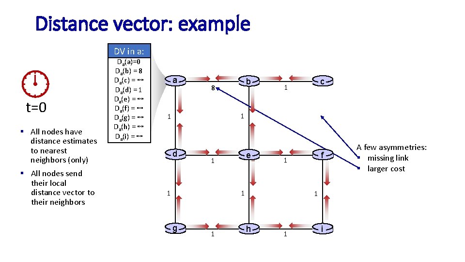
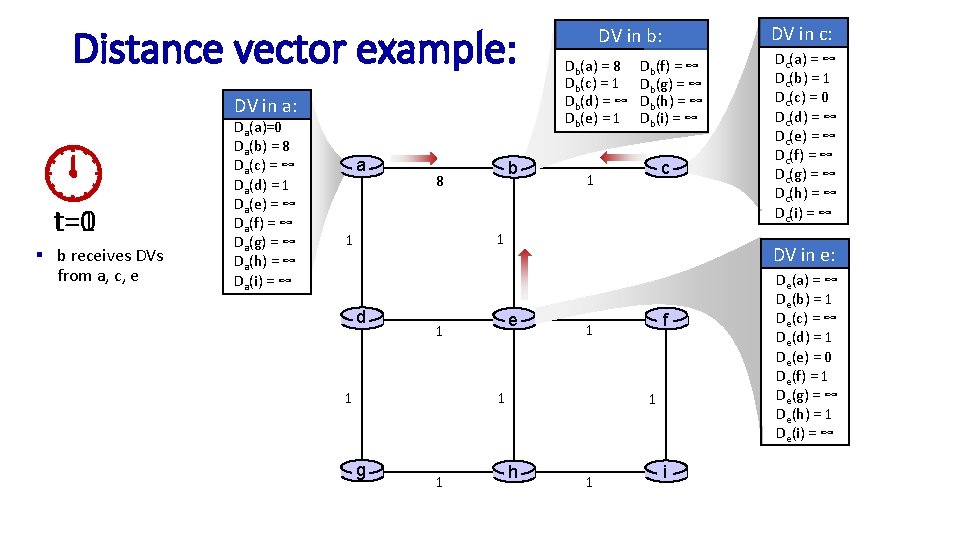
Distance vector: example DV in a: t=0 § All nodes have distance estimates to nearest neighbors (only) § All nodes send their local distance vector to their neighbors Da(a)=0 Da(b) = 8 Da(c) = ∞ Da(d) = 1 Da(e) = ∞ Da(f) = ∞ Da(g) = ∞ Da(h) = ∞ Da(i) = ∞ a b 8 c 1 1 1 d e 1 1 1 g 1 f 1 1 h 1 i A few asymmetries: § missing link § larger cost

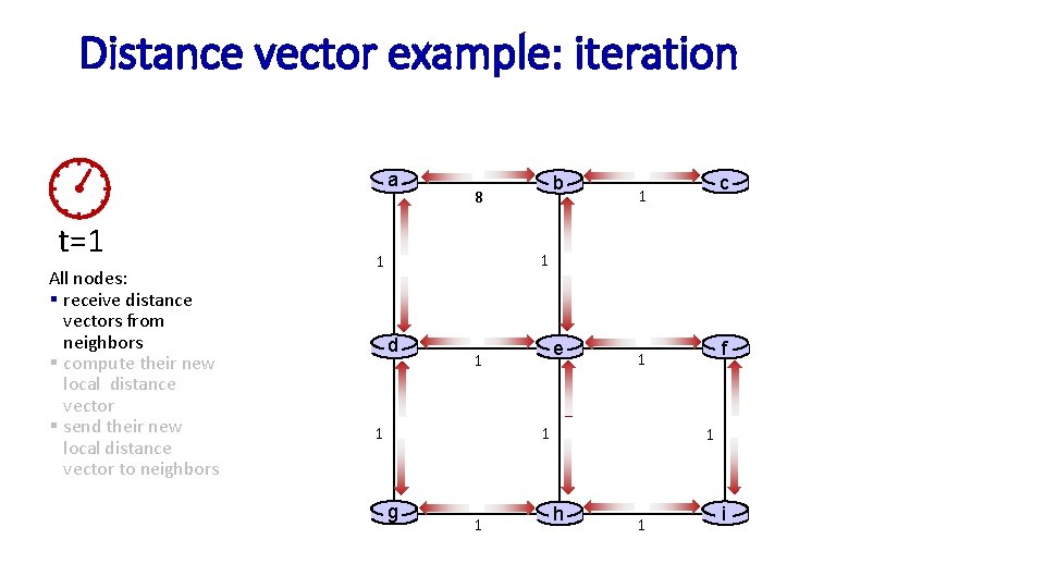
Distance vector example: iteration a t=1 All nodes: § receive distance vectors from neighbors § compute their new local distance vector § send their new local distance vector to neighbors b 8 c 1 1 1 d e 1 1 1 g 1 f 1 1 h 1 i

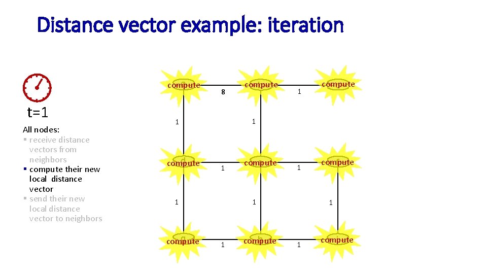
Distance vector example: iteration a compute t=1 All nodes: § receive distance vectors from neighbors § compute their new local distance vector § send their new local distance vector to neighbors 8 1 1 g compute 1 compute c 1 1 d compute b e compute 1 1 1 h compute f 1 1 i compute

Distance vector example: iteration a t=1 All nodes: § receive distance vectors from neighbors § compute their new local distance vector § send their new local distance vector to neighbors b 8 c 1 1 1 d e 1 1 1 g 1 f 1 1 h 1 i

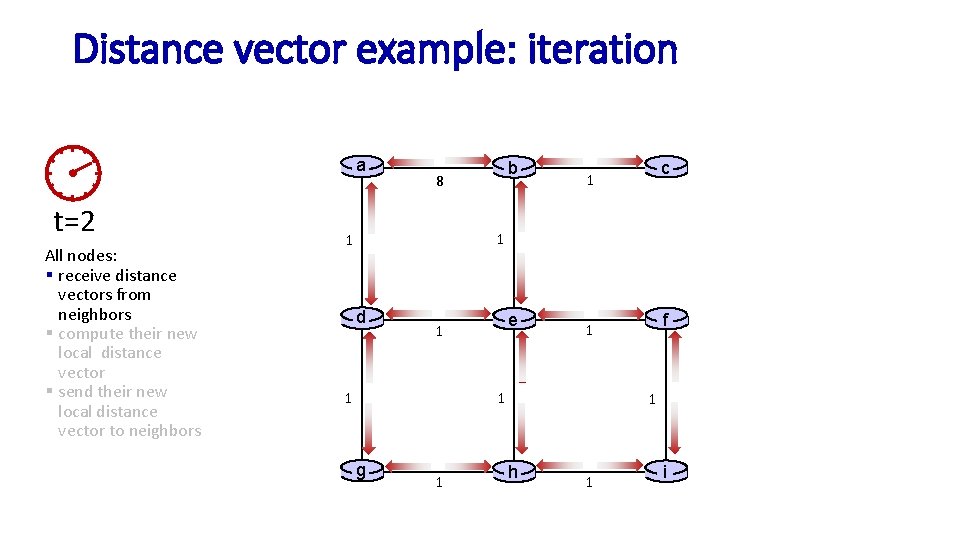
Distance vector example: iteration a t=2 All nodes: § receive distance vectors from neighbors § compute their new local distance vector § send their new local distance vector to neighbors b 8 c 1 1 1 d e 1 1 1 g 1 f 1 1 h 1 i

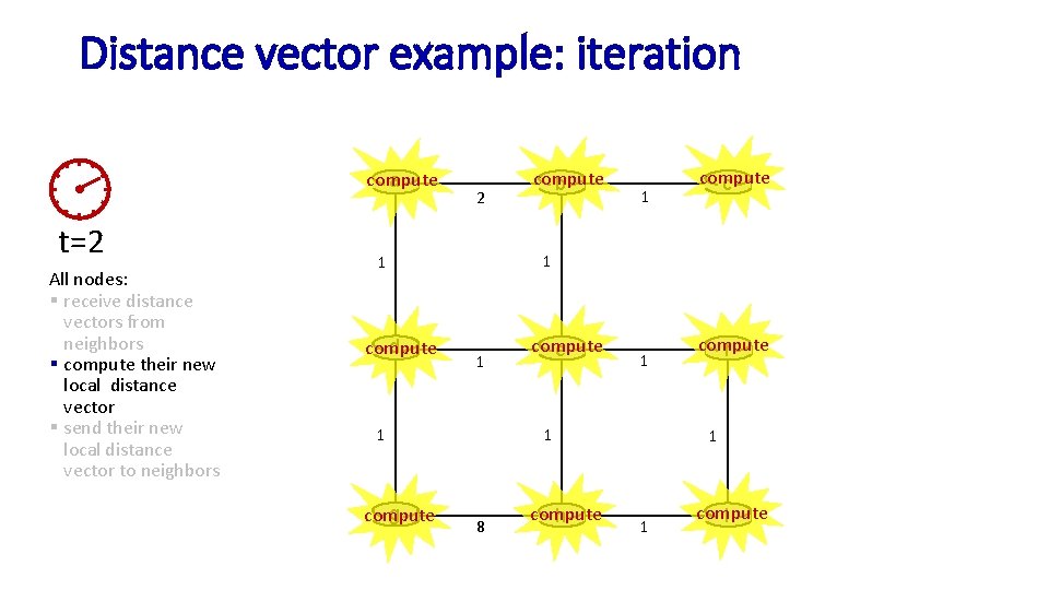
Distance vector example: iteration compute a t=2 All nodes: § receive distance vectors from neighbors § compute their new local distance vector § send their new local distance vector to neighbors 2 1 1 g compute 1 compute c 1 1 d compute b compute e 1 1 8 compute h compute f 1 1 compute i

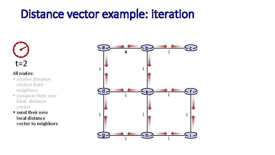
Distance vector example: iteration a t=2 All nodes: § receive distance vectors from neighbors § compute their new local distance vector § send their new local distance vector to neighbors b 8 c 1 1 1 d e 1 1 1 g 1 f 1 1 h 1 i

Distance vector example: iteration …. and so on Let’s next take a look at the iterative computations at nodes

Distance vector example: computation DV in b: Db(a) = 8 Db(c) = 1 Db(d) = ∞ Db(e) = 1 DV in a: t=1 t=0 § b receives DVs from a, c, e Da(a)=0 Da(b) = 8 Da(c) = ∞ Da(d) = 1 Da(e) = ∞ Da(f) = ∞ Da(g) = ∞ Da(h) = ∞ Da(i) = ∞ a b 8 Db(f) = ∞ Db(g) = ∞ Db(h) = ∞ Db(i) = ∞ c 1 1 1 d 1 1 f 1 1 g Dc(a) = ∞ Dc(b) = 1 Dc(c) = 0 Dc(d) = ∞ Dc(e) = ∞ Dc(f) = ∞ Dc(g) = ∞ Dc(h) = ∞ Dc(i) = ∞ DV in e: e 1 DV in c: 1 h 1 i De(a) = ∞ De(b) = 1 De(c) = ∞ De(d) = 1 De(e) = 0 De(f) = 1 De(g) = ∞ De(h) = 1 De(i) = ∞

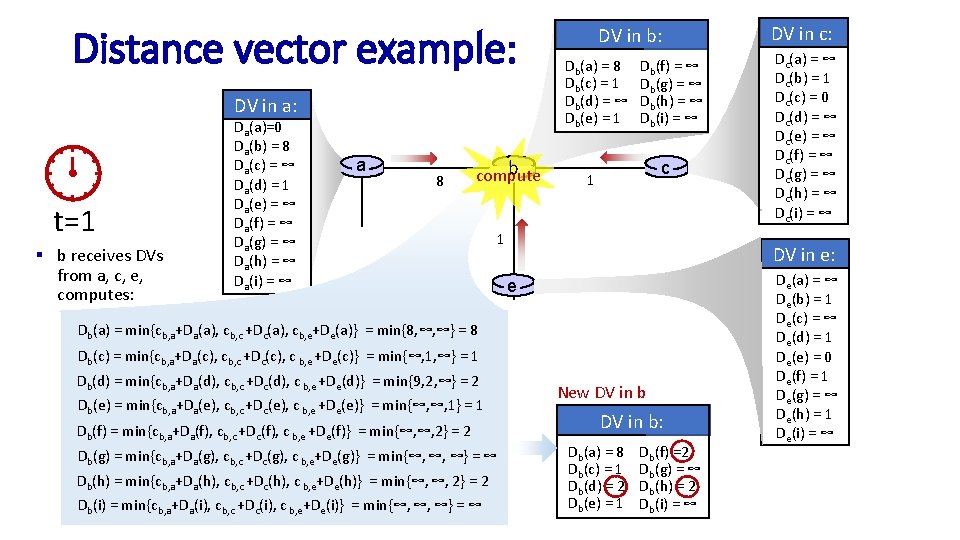
Distance vector example: computation DV in b: Db(a) = 8 Db(c) = 1 Db(d) = ∞ Db(e) = 1 DV in a: t=1 § b receives DVs from a, c, e, computes: Da(a)=0 Da(b) = 8 Da(c) = ∞ Da(d) = 1 Da(e) = ∞ Da(f) = ∞ Da(g) = ∞ Da(h) = ∞ Da(i) = ∞ a 8 b compute Db(f) = ∞ Db(g) = ∞ Db(h) = ∞ Db(i) = ∞ c 1 1 1 d e f 1 Db(c) = min{cb, a+Da(c), cb, c +Dc(c), c b, e +De(c)} = min{∞, 1, ∞} = 1 Db(d) = min{cb, a+Da(d), cb, c +Dc(d), c b, e +De(d)} = min{9, 2, ∞} = 2 1 1 Db(e) = min{cb, a+Da(e), cb, c +Dc(e), c b, e +De(e)} = min{∞, ∞, 1} = 1 New DV in b 1 DV in b: Db(f) = min{cb, a+Da(f), cb, c +Dc(f), c b, e +De(f)} = min{∞, ∞, 2} = 2 Db(g) = min{cb, a+Da(g), cb, c +Dc(g), c b, e+De(g)} = min{∞, ∞, ∞} = ∞ g 1 ∞, 2} = 2 Db(h) = min{cb, a+Da(h), cb, c +Dc(h), c b, e+De(h)} = min{∞, Db(i) = min{cb, a+Da(i), cb, c +Dc(i), c b, e+De(i)} = min{∞, ∞, ∞} = ∞ Dc(a) = ∞ Dc(b) = 1 Dc(c) = 0 Dc(d) = ∞ Dc(e) = ∞ Dc(f) = ∞ Dc(g) = ∞ Dc(h) = ∞ Dc(i) = ∞ DV in e: e 1 Db(a) = min{cb, a+Da(a), cb, c +Dc(a), cb, e+De(a)} = min{8, ∞, ∞} =8 DV in c: h Db(a) = 8 D (c) = 1 1 Db(d) = 2 b Db(e) = 1 Db(f) =2 Db(g) i =∞ Db(h) = 2 Db(i) = ∞ De(a) = ∞ De(b) = 1 De(c) = ∞ De(d) = 1 De(e) = 0 De(f) = 1 De(g) = ∞ De(h) = 1 De(i) = ∞

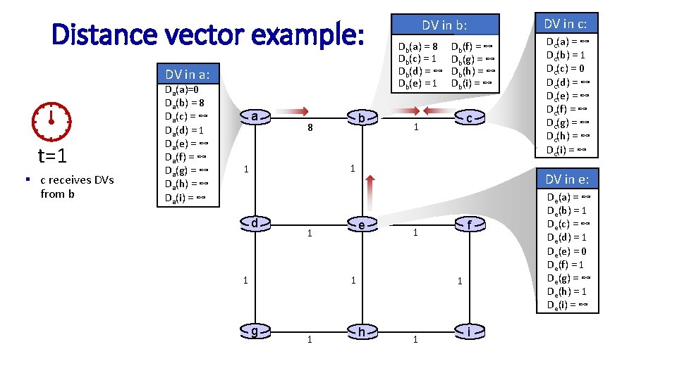
Distance vector example: computation DV in b: Db(a) = 8 Db(c) = 1 Db(d) = ∞ Db(e) = 1 DV in a: t=1 § c receives DVs from b Da(a)=0 Da(b) = 8 Da(c) = ∞ Da(d) = 1 Da(e) = ∞ Da(f) = ∞ Da(g) = ∞ Da(h) = ∞ Da(i) = ∞ a b 8 Db(f) = ∞ Db(g) = ∞ Db(h) = ∞ Db(i) = ∞ c 1 1 1 d 1 1 f 1 1 g Dc(a) = ∞ Dc(b) = 1 Dc(c) = 0 Dc(d) = ∞ Dc(e) = ∞ Dc(f) = ∞ Dc(g) = ∞ Dc(h) = ∞ Dc(i) = ∞ DV in e: e 1 DV in c: 1 h 1 i De(a) = ∞ De(b) = 1 De(c) = ∞ De(d) = 1 De(e) = 0 De(f) = 1 De(g) = ∞ De(h) = 1 De(i) = ∞

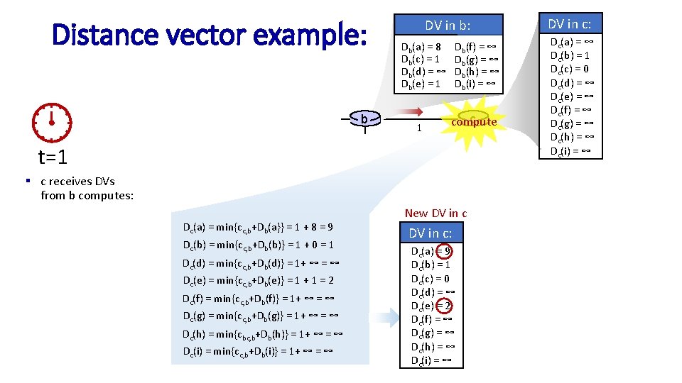
Distance vector example: computation DV in b: Db(a) = 8 Db(c) = 1 Db(d) = ∞ Db(e) = 1 a t=1 § c receives DVs from b computes: b 8 1 d b(a}} = 1 + 8 = 9 Dc(a) = min{cc, b+D c compute 1 e Dc(b) = min{cc, b+Db(b)} = 1 + 0 = 1 Dc(d) = min{cc, b+Db(d)} = 1+ ∞ = ∞ Dc(e) = min{cc, b+Db(e)} = 1 + 1 = 2 Dc(f) = min{cc, b+Db(f)} = 1+ ∞ = ∞ Dc(g) = min{cc, b+Db(g)} = 1+ ∞ = ∞ Dc(h) = min{cbc, bg+Db(h)} = 1+ ∞ = ∞ Dc(i) = min{cc, b+Db(i)} = 1+ ∞ = ∞ 1 Db(f) = ∞ Db(g) = ∞ Db(h) = ∞ Db(i) = ∞ h New DV in c: Dc(a) = 9 Dc(b) = 1 Dc(c) = 0 Dc(d) = ∞ Dc(e) = 2 Dc(f) = ∞ Dc(g) = ∞ Dc(h) = ∞ Dc(i) = ∞ f i DV in c: Dc(a) = ∞ Dc(b) = 1 Dc(c) = 0 Dc(d) = ∞ Dc(e) = ∞ Dc(f) = ∞ Dc(g) = ∞ Dc(h) = ∞ Dc(i) = ∞

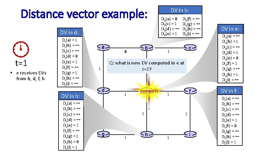
Distance vector example: computation DV in b: Db(a) = 8 Db(c) = 1 Db(d) = ∞ Db(e) = 1 DV in d: t=1 § e receives DVs from b, d, f, h Dc(a) = 1 Dc(b) = ∞ Dc(c) = ∞ Dc(d) = 0 Dc(e) = 1 Dc(f) = ∞ Dc(g) = 1 Dc(h) = ∞ Dc(i) = ∞ a Dc(a) = ∞ Dc(b) = ∞ Dc(c) = ∞ Dc(d) = ∞ Dc(e) = 1 Dc(f) = ∞ Dc(g) = 1 Dc(h) = 0 Dc(i) = 1 c 1 Q: what is new DV computed in e at 1 t=1? 1 d DV in h: b 8 Db(f) = ∞ Db(g) = ∞ Db(h) = ∞ Db(i) = ∞ 1 1 compute e 1 g 1 f 1 1 h 1 i DV in e: De(a) = ∞ De(b) = 1 De(c) = ∞ De(d) = 1 De(e) = 0 De(f) = 1 De(g) = ∞ De(h) = 1 De(i) = ∞ DV in f: Dc(a) = ∞ Dc(b) = ∞ Dc(c) = ∞ Dc(d) = ∞ Dc(e) = 1 Dc(f) = 0 Dc(g) = ∞ Dc(h) = ∞ Dc(i) = 1

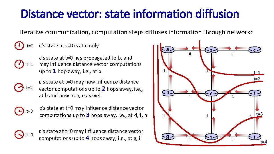
Distance vector: state information diffusion Iterative communication, computation steps diffuses information through network: t=0 t=1 t=2 c’s state at t=0 is at c only c’s state at t=0 has propagated to b, and may influence distance vector computations up to 1 hop away, i. e. , at b a t=3 c’s state at t=0 may influence distance vector computations up to 3 hops away, i. e. , at d, f, h t=4 c’s state at t=0 may influence distance vector computations up to 4 hops away, i. e. , at g, i 1 1 1 c’s state at t=0 may now influence distance vector computations up to 2 hops away, i. e. , at b and now at a, e as well b 8 d 1 t=2 e 1 1 1 f 1 t=3 1 g c h 1 i t=4

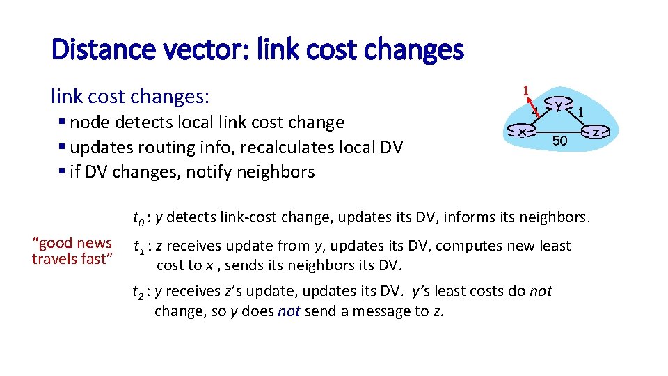
Distance vector: link cost changes: § node detects local link cost change § updates routing info, recalculates local DV § if DV changes, notify neighbors 1 x y 4 1 50 t 0 : y detects link-cost change, updates its DV, informs its neighbors. “good news travels fast” t 1 : z receives update from y, updates its DV, computes new least cost to x , sends its neighbors its DV. t 2 : y receives z’s update, updates its DV. y’s least costs do not change, so y does not send a message to z. z

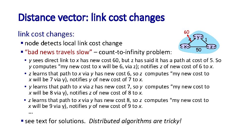
Distance vector: link cost changes: § node detects local link cost change § “bad news travels slow” – count-to-infinity problem: 60 x 4 y 50 1 z • y sees direct link to x has new cost 60, but z has said it has a path at cost of 5. So y computes “my new cost to x will be 6, via z); notifies z of new cost of 6 to x. • z learns that path to x via y has new cost 6, so z computes “my new cost to x will be 7 via y), notifies y of new cost of 7 to x. • y learns that path to x via z has new cost 7, so y computes “my new cost to x will be 8 via y), notifies z of new cost of 8 to x. • z learns that path to x via y has new cost 8, so z computes “my new cost to x will be 9 via y), notifies y of new cost of 9 to x. … § see text for solutions. Distributed algorithms are tricky!

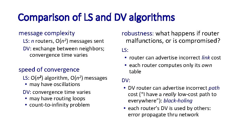
Comparison of LS and DV algorithms message complexity LS: n routers, O(n 2) messages sent DV: exchange between neighbors; convergence time varies speed of convergence LS: O(n 2) algorithm, O(n 2) messages • may have oscillations DV: convergence time varies • may have routing loops • count-to-infinity problem robustness: what happens if router malfunctions, or is compromised? LS: • router can advertise incorrect link cost • each router computes only its own table DV: • DV router can advertise incorrect path cost (“I have a really low-cost path to everywhere”): black-holing • each router’s DV is used by others: error propagate thru network