Network Layer contd Routing Packet transfer in network

Network Layer (contd. ) Routing

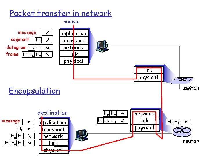
Packet transfer in network source message segment Ht M datagram Hn Ht M frame Hl Hn Ht M M application transport network link physical switch Encapsulation destination message M Ht M Hn Ht Hl Hn Ht M M application transport network link physical Hn Ht Hl Hn Ht M M network link physical Hn Ht M router

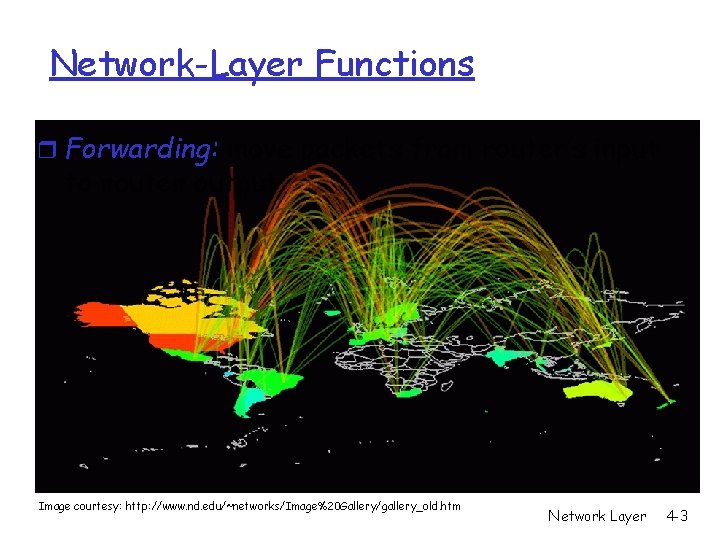
Network-Layer Functions r Forwarding: move packets from router’s input to router output Image courtesy: http: //www. nd. edu/~networks/Image%20 Gallery/gallery_old. htm Network Layer 4 -3

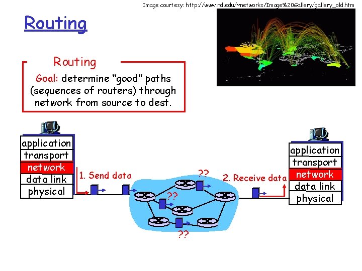
Image courtesy: http: //www. nd. edu/~networks/Image%20 Gallery/gallery_old. htm Routing Goal: determine “good” paths (sequences of routers) through network from source to dest. application transport network data link 1. Send data physical ? ? ? application transport 2. Receive data network data link physical

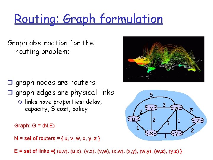
Routing: Graph formulation Graph abstraction for the routing problem: r graph nodes are routers r graph edges are physical links m links have properties: delay, capacity, $ cost, policy Graph: G = (N, E) N = set of routers = { u, v, w, x, y, z } 5 2 u v 2 1 x 3 w 3 1 5 z 1 y E = set of links ={ (u, v), (u, x), (v, w), (x, y), (w, z), (y, z) } 2

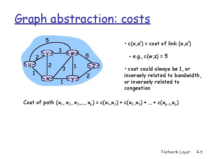
Graph abstraction: costs 5 2 u v 2 1 x • c(x, x’) = cost of link (x, x’) 3 w 3 1 5 z 1 y - e. g. , c(w, z) = 5 2 • cost could always be 1, or inversely related to bandwidth, or inversely related to congestion Cost of path (x 1, x 2, x 3, …, xp) = c(x 1, x 2) + c(x 2, x 3) + … + c(xp-1, xp) Network Layer 4 -6

Key Desired Properties of a Routing Algorithm r Simplicity r Robustness r Optimality m find good path (for user/provider) 7

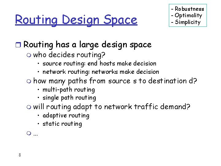
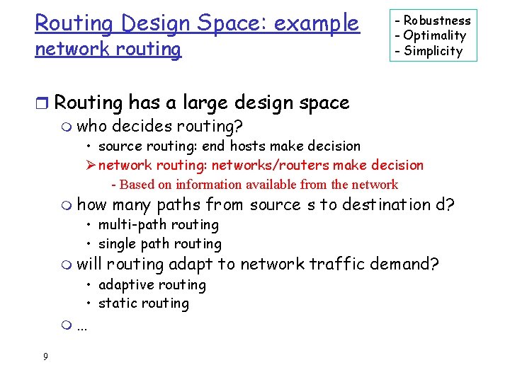
Routing Design Space - Robustness - Optimality - Simplicity r Routing has a large design space m who decides routing? • source routing: end hosts make decision • network routing: networks make decision m how many paths from source s to destination d? • multi-path routing • single path routing m will routing adapt to network traffic demand? • adaptive routing • static routing m… 8

Routing Design Space: example network routing - Robustness - Optimality - Simplicity r Routing has a large design space m who decides routing? • source routing: end hosts make decision Ø network routing: networks/routers make decision - Based on information available from the network m how many paths from source s to destination d? • multi-path routing • single path routing m will routing adapt to network traffic demand? • adaptive routing • static routing m… 9

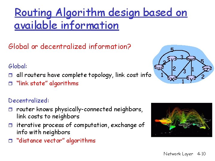
Routing Algorithm design based on available information Global or decentralized information? Global: r all routers have complete topology, link cost info r “link state” algorithms 5 u 2 1 v 2 x 3 3 1 w 1 y 5 2 z Decentralized: r router knows physically-connected neighbors, link costs to neighbors r iterative process of computation, exchange of info with neighbors r “distance vector” algorithms Network Layer 4 -10

Link state (LS) routing algorithm Network Layer 4 -11

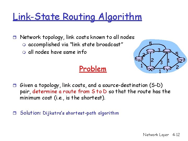
Link-State Routing Algorithm r Network topology, link costs known to all nodes m m 5 accomplished via “link state broadcast” all nodes have same info u Problem 2 1 v 2 x 3 3 1 w 1 y 5 2 z r Given a topology, link costs, and a source-destination (S-D) pair, determine a route from S to D so that the route has the minimum cost (i. e. , is the shortest). r Solution: Dijkstra’s shortest-path algorithm Network Layer 4 -12

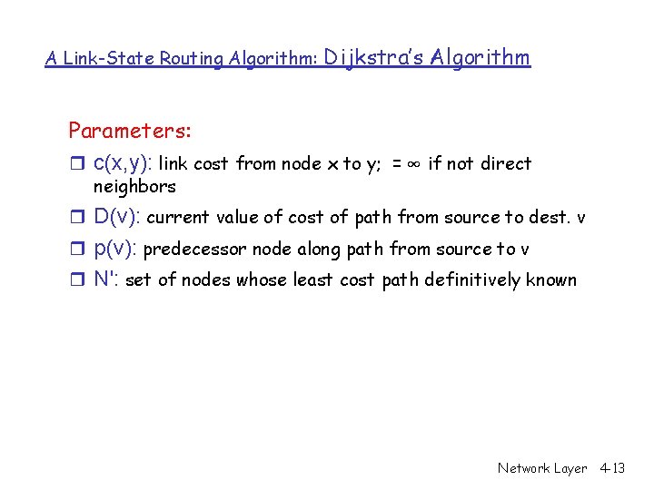
A Link-State Routing Algorithm: Dijkstra’s Algorithm Parameters: r c(x, y): link cost from node x to y; = ∞ if not direct neighbors r D(v): current value of cost of path from source to dest. v r p(v): predecessor node along path from source to v r N': set of nodes whose least cost path definitively known Network Layer 4 -13

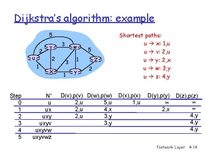
Dijkstra’s algorithm: example 5 2 u 2 1 Step 0 1 2 3 4 5 v x N' u ux uxyvwz 3 w 3 1 5 z 1 y 2 D(v), p(v) D(w), p(w) 2, u 5, u 2, u 4, x 2, u 3, y Shortest paths: u x: 1, u u v: 2, u u y: 2, x u w: 3, y u z: 4, y D(x), p(x) 1, u D(y), p(y) ∞ 2, x D(z), p(z) ∞ ∞ 4, y Network Layer 4 -14

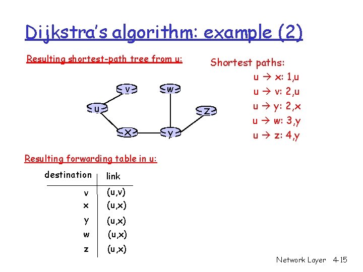
Dijkstra’s algorithm: example (2) Resulting shortest-path tree from u: v w x y u Shortest paths: u x: 1, u u v: 2, u u y: 2, x z u w: 3, y u z: 4, y Resulting forwarding table in u: destination link v x (u, v) (u, x) y (u, x) w (u, x) z (u, x) Network Layer 4 -15

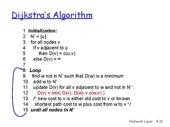
Dijkstra’s Algorithm 1 Initialization: 2 N' = {u} 3 for all nodes v 4 if v adjacent to u 5 then D(v) = c(u, v) 6 else D(v) = ∞ 7 8 Loop 9 find w not in N' such that D(w) is a minimum 10 add w to N' 11 update D(v) for all v adjacent to w and not in N' : 12 D(v) = min( D(v), D(w) + c(w, v) ) 13 /* new cost to v is either old cost to v or known 14 shortest path cost to w plus cost from w to v */ 15 until all nodes in N' Network Layer 4 -16

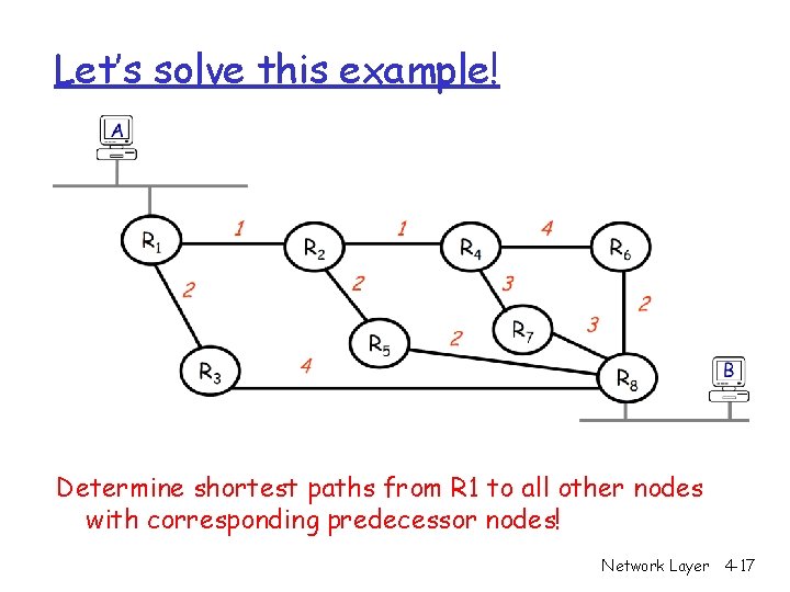
Let’s solve this example! Determine shortest paths from R 1 to all other nodes with corresponding predecessor nodes! Network Layer 4 -17

Distance Vector routing algorithm Network Layer 4 -18

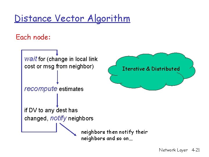
Distance Vector Routing r Practically entire network topology (each link state) may not be known accurately m Only the information to a direct neighbor may be known r Distance-vector routing algorithm operates by m Each router trusting its direct neighbors m Each router maintain a table (vector) estimating • the best known distance to each destination • which line to use to get there m Tables (vectors) are updated by exchanging information with the direct neighbors

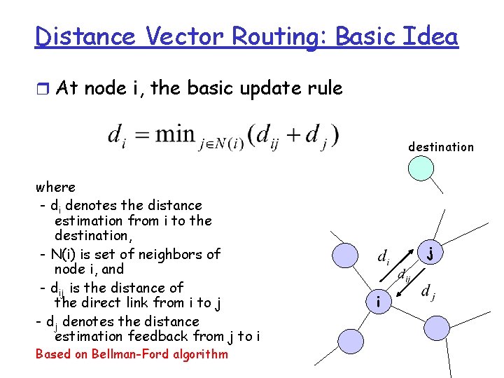
Distance Vector Routing: Basic Idea r At node i, the basic update rule destination where - di denotes the distance estimation from i to the destination, - N(i) is set of neighbors of node i, and - dij is the distance of the direct link from i to j - dj denotes the distance estimation feedback from j to i Based on Bellman-Ford algorithm j i

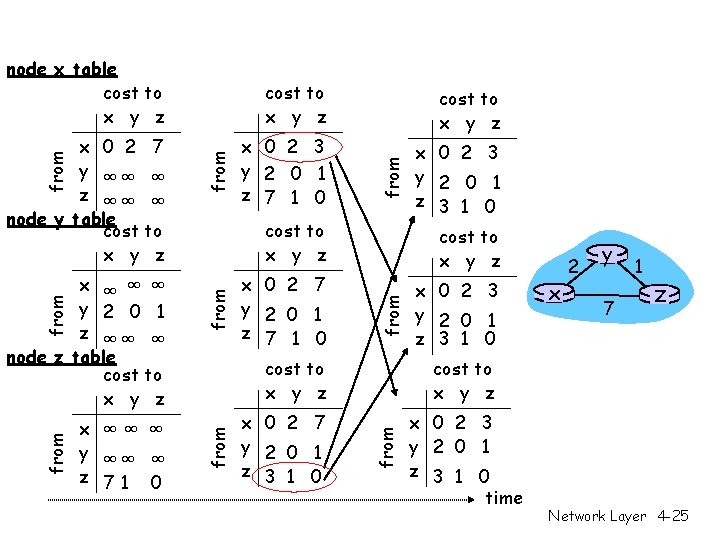
Distance Vector Algorithm Each node: wait for (change in local link cost or msg from neighbor) Iterative & Distributed recompute estimates if DV to any dest has changed, notify neighbors then notify their neighbors and so on… Network Layer 4 -21

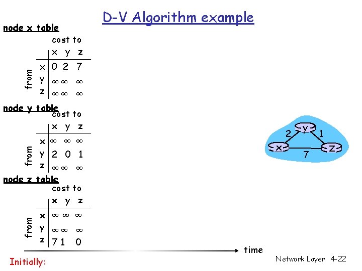
from node x table cost to x y z D-V Algorithm example x 0 2 7 y ∞∞ ∞ z ∞∞ ∞ node y table cost to x y z x ∞ ∞ ∞ y 2 0 1 z ∞∞ ∞ node z table cost to x y z from x x ∞∞ ∞ y ∞∞ ∞ z 71 0 Initially: time 2 y 7 1 z Network Layer 4 -22

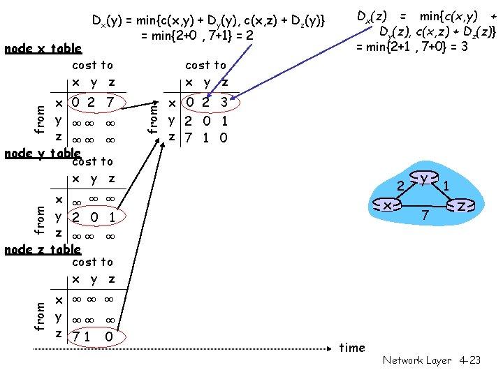
Dx(y) = min{c(x, y) + Dy(y), c(x, z) + Dz(y)} = min{2+0 , 7+1} = 2 node x table cost to x y z from x 0 2 7 y ∞∞ ∞ z ∞∞ ∞ node y table cost to x y z Dx(z) = min{c(x, y) + Dy(z), c(x, z) + Dz(z)} = min{2+1 , 7+0} = 3 x 0 2 3 y 2 0 1 z 7 1 0 x ∞ ∞ ∞ y 2 0 1 z ∞∞ ∞ node z table cost to x y z from x x ∞∞ ∞ y ∞∞ ∞ z 71 0 time 2 y 7 1 z Network Layer 4 -23

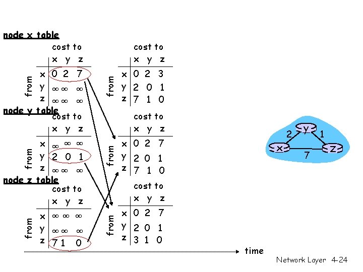
node x table cost to x y z from x ∞∞ ∞ y ∞∞ ∞ z 71 0 from x ∞ ∞ ∞ y 2 0 1 z ∞∞ ∞ node z table cost to x y z x 0 2 3 y 2 0 1 z 7 1 0 cost to x y z x 0 2 7 y 2 0 1 z 7 1 0 x 2 y 7 1 z cost to x y z from x 0 2 7 y ∞∞ ∞ z ∞∞ ∞ node y table cost to x y z x 0 2 7 y 2 0 1 z 3 1 0 time Network Layer 4 -24

node x table cost to x y z x ∞∞ ∞ y ∞∞ ∞ z 71 0 from x 0 2 7 y 2 0 1 z 7 1 0 cost to x y z x 0 2 7 y 2 0 1 z 3 1 0 x 0 2 3 y 2 0 1 z 3 1 0 cost to x y z x 0 2 3 y 2 0 1 z 3 1 0 x 2 y 7 1 z cost to x y z from x ∞ ∞ ∞ y 2 0 1 z ∞∞ ∞ node z table cost to x y z x 0 2 3 y 2 0 1 z 7 1 0 cost to x y z from x 0 2 7 y ∞∞ ∞ z ∞∞ ∞ node y table cost to x y z x 0 2 3 y 2 0 1 z 3 1 0 time Network Layer 4 -25

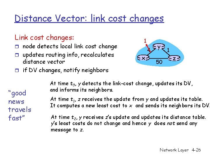
Distance Vector: link cost changes Link cost changes: r node detects local link cost change r updates routing info, recalculates distance vector r if DV changes, notify neighbors “good news travels fast” 1 x 4 y 50 1 z At time t 0, y detects the link-cost change, updates its DV, and informs its neighbors. At time t 1, z receives the update from y and updates its table. It computes a new least cost to x and sends its neighbors its DV. At time t 2, y receives z’s update and updates its distance table. y’s least costs do not change and hence y does not send any message to z. Network Layer 4 -26

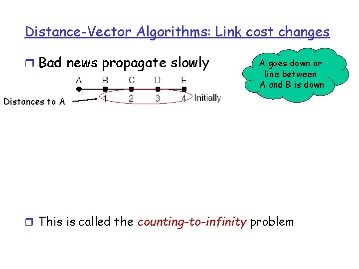
Distance-Vector Algorithms: Link cost changes r Bad news propagate slowly A goes down or line between A and B is down Distances to A r This is called the counting-to-infinity problem

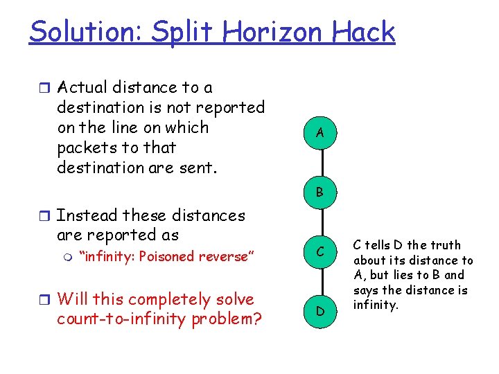
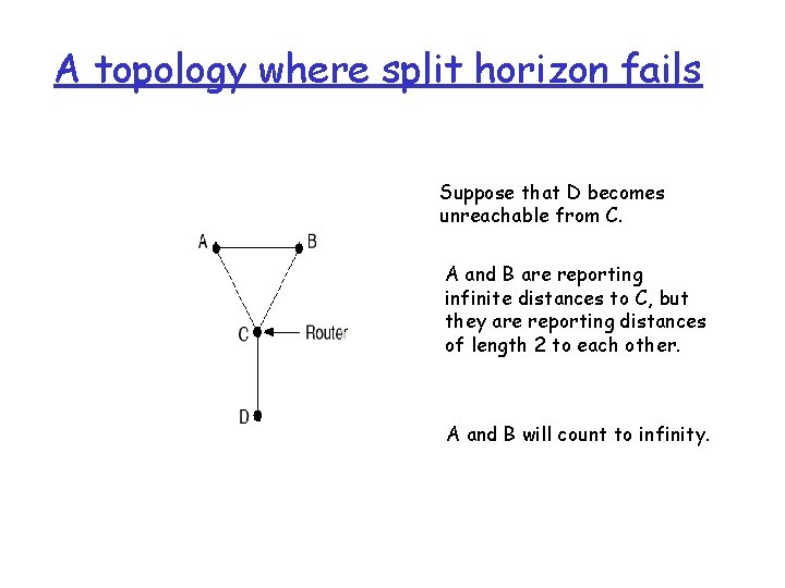
Solution: Split Horizon Hack r Actual distance to a destination is not reported on the line on which packets to that destination are sent. A B r Instead these distances are reported as m “infinity: Poisoned reverse” r Will this completely solve count-to-infinity problem? C D C tells D the truth about its distance to A, but lies to B and says the distance is infinity.

A topology where split horizon fails Suppose that D becomes unreachable from C. A and B are reporting infinite distances to C, but they are reporting distances of length 2 to each other. A and B will count to infinity.

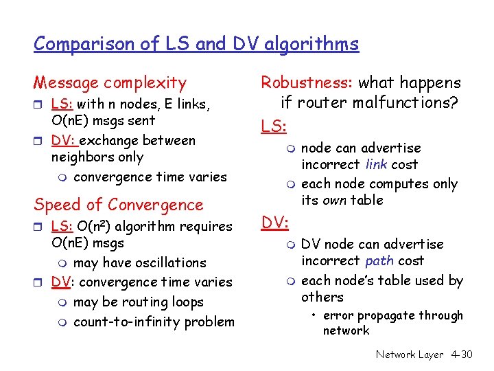
Comparison of LS and DV algorithms Message complexity r LS: with n nodes, E links, O(n. E) msgs sent r DV: exchange between neighbors only m convergence time varies Speed of Convergence r LS: O(n 2) algorithm requires O(n. E) msgs m may have oscillations r DV: convergence time varies m may be routing loops m count-to-infinity problem Robustness: what happens if router malfunctions? LS: m m node can advertise incorrect link cost each node computes only its own table DV: m m DV node can advertise incorrect path cost each node’s table used by others • error propagate through network Network Layer 4 -30