
Network Data Visualization Neal Patwari Assistant Professor Dept


- Slides: 36
Network Data Visualization Neal Patwari Assistant Professor Dept of Electrical & Computer Engineering http: //span. ece. utah. edu CS 5480/6480 - Computer Networks 14 October 2007
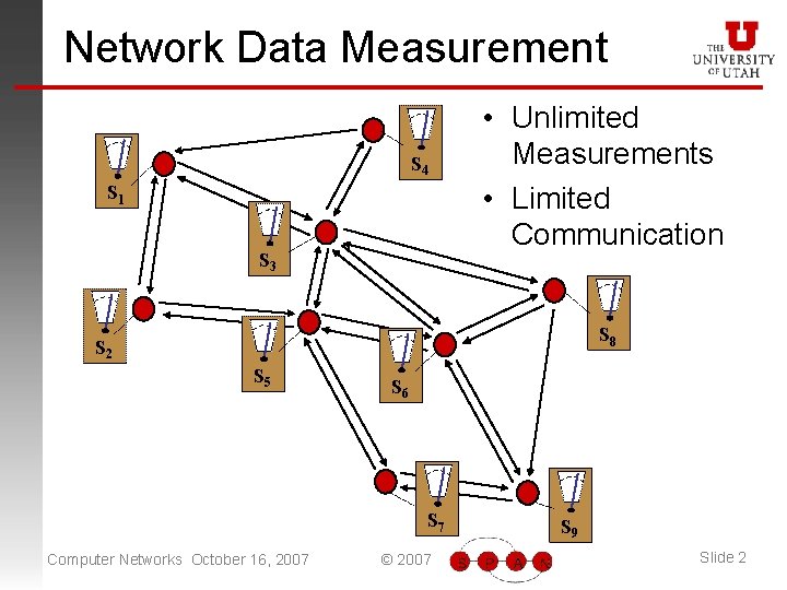
Network Data Measurement S 4 S 1 S 3 • Unlimited Measurements • Limited Communication S 8 S 2 S 5 S 6 S 7 Computer Networks October 16, 2007 © 2007 S 9 Slide 2
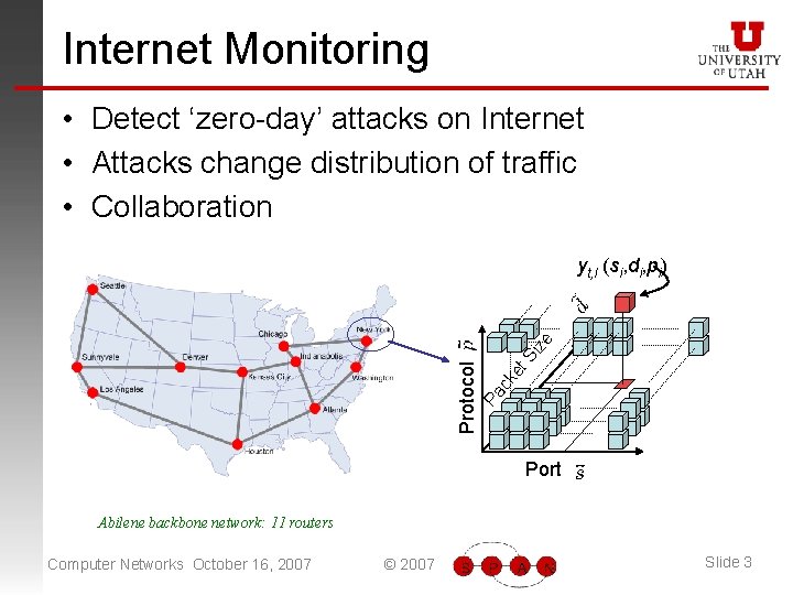
Internet Monitoring • Detect ‘zero-day’ attacks on Internet • Attacks change distribution of traffic • Collaboration S et ck Pa Protocol ize yt, l (si, di, pi) Port Abilene backbone network: 11 routers Computer Networks October 16, 2007 © 2007 Slide 3
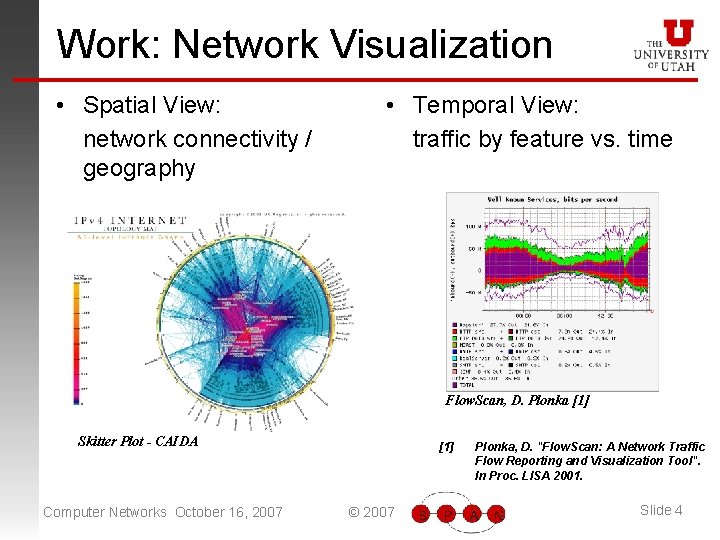
Work: Network Visualization • Spatial View: network connectivity / geography • Temporal View: traffic by feature vs. time Flow. Scan, D. Plonka [1] Skitter Plot - CAIDA Computer Networks October 16, 2007 [1] © 2007 Plonka, D. "Flow. Scan: A Network Traffic Flow Reporting and Visualization Tool". In Proc. LISA 2001. Slide 4
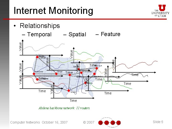
Internet Monitoring • Relationships Time Value Value Time Value Time – Feature – Spatial Value – Temporal Time Time Abilene backbone network: 11 routers Computer Networks October 16, 2007 © 2007 Slide 5
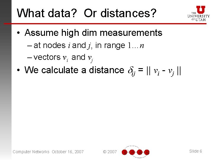
What data? Or distances? • Assume high dim measurements – at nodes i and j, in range 1…n – vectors vi and vj • We calculate a distance dij = || vi - vj || Computer Networks October 16, 2007 © 2007 Slide 6
Outline • Manifold Learning and Dimension Reduction • Map-tools Operation • Map-tools Example Computer Networks October 16, 2007 © 2007 Slide 7
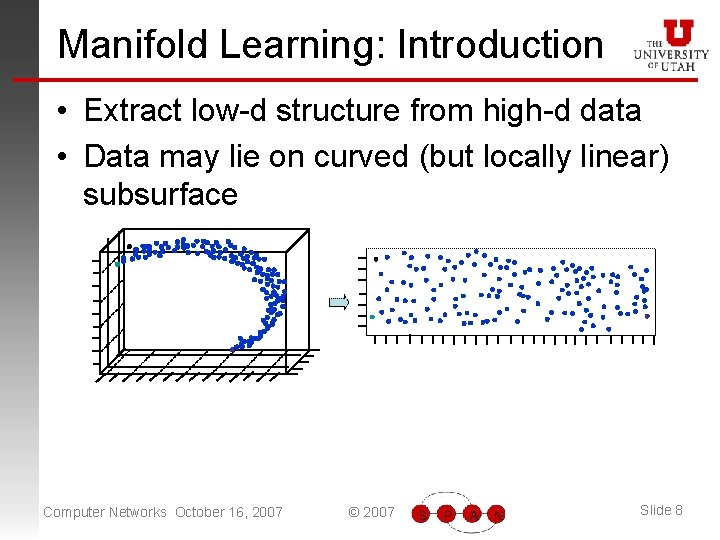
Manifold Learning: Introduction • Extract low-d structure from high-d data • Data may lie on curved (but locally linear) subsurface Computer Networks October 16, 2007 © 2007 Slide 8
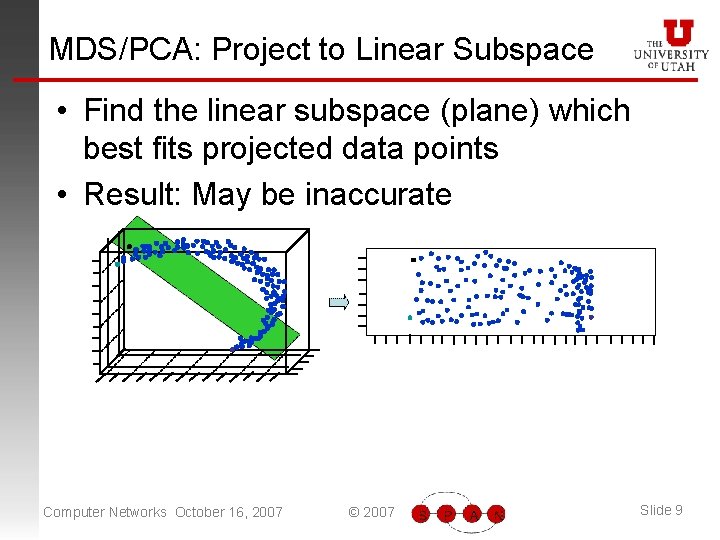
MDS/PCA: Project to Linear Subspace • Find the linear subspace (plane) which best fits projected data points • Result: May be inaccurate Computer Networks October 16, 2007 © 2007 Slide 9
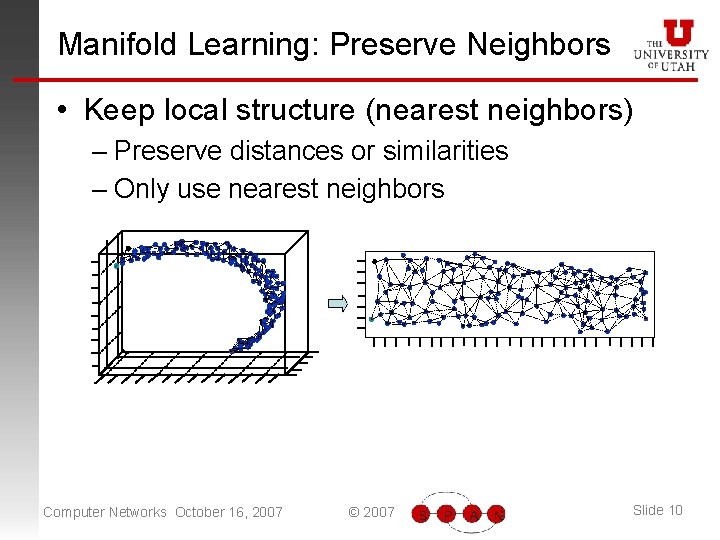
Manifold Learning: Preserve Neighbors • Keep local structure (nearest neighbors) – Preserve distances or similarities – Only use nearest neighbors Computer Networks October 16, 2007 © 2007 Slide 10
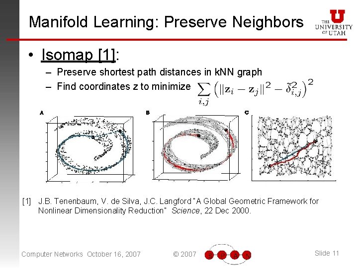
Manifold Learning: Preserve Neighbors • Isomap [1]: – Preserve shortest path distances in k. NN graph – Find coordinates z to minimize [1] J. B. Tenenbaum, V. de Silva, J. C. Langford “A Global Geometric Framework for Nonlinear Dimensionality Reduction” Science, 22 Dec 2000. Computer Networks October 16, 2007 © 2007 Slide 11
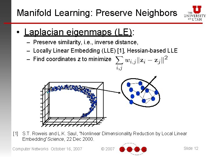
Manifold Learning: Preserve Neighbors • Laplacian eigenmaps (LE): – Preserve similarity, i. e. , inverse distance, – Locally Linear Embedding (LLE) [1], Hessian-based LLE – Find coordinates z to minimize [1] S. T. Roweis and L. K. Saul, "Nonlinear Dimensionality Reduction by Local Linear Embedding“Science, 22 Dec 2000. Computer Networks October 16, 2007 © 2007 Slide 12
Manifold Learning: Preserve Neighbors • Weighted multi-dimensional scaling (WMDS): – Preserve weighted dist (weight = 0 for non-neighbors) – Find coordinates z to minimize • Pair (i, j) weight: Prior for i weight: – Non-incr. cost: majorization, computation O(k) – Local communication, measurement [12] J. Costa, N. Patwari, A. O. Hero III “Distributed Weighted Multidimensional Scaling for Node Localization in Sensor Networks”, IEEE/ACM Trans. Sensor Networks, Feb. 2006. Computer Networks October 16, 2007 © 2007 Slide 13
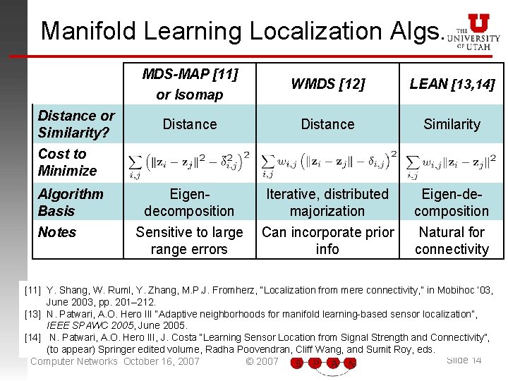
Manifold Learning Localization Algs. Distance or Similarity? MDS-MAP [11] or Isomap WMDS [12] LEAN [13, 14] Distance Similarity Eigendecomposition Iterative, distributed majorization Eigen-decomposition Cost to Minimize Algorithm Basis Notes Sensitive to large Can incorporate prior range errors info Natural for connectivity [11] Y. Shang, W. Ruml, Y. Zhang, M. P. J. Fromherz, “Localization from mere connectivity, ” in Mobihoc ’ 03, June 2003, pp. 201– 212. [13] N. Patwari, A. O. Hero III “Adaptive neighborhoods for manifold learning-based sensor localization”, IEEE SPAWC 2005, June 2005. [14] N. Patwari, A. O. Hero III, J. Costa “Learning Sensor Location from Signal Strength and Connectivity”, (to appear) Springer edited volume, Radha Poovendran, Cliff Wang, and Sumit Roy, eds. Slide 14 Computer Networks October 16, 2007 © 2007
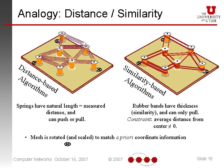
Analogy: Distance / Similarity Di sta Al ncego rith base ms d Sim ila Al rity go -b rith ase ms d Springs have natural length = measured distance, and can push or pull. Rubber bands have thickness (similarity), and can only pull. Constraint: average distance from center ≠ 0. • Mesh is rotated (and scaled) to match a priori coordinate information Computer Networks October 16, 2007 © 2007 Slide 15
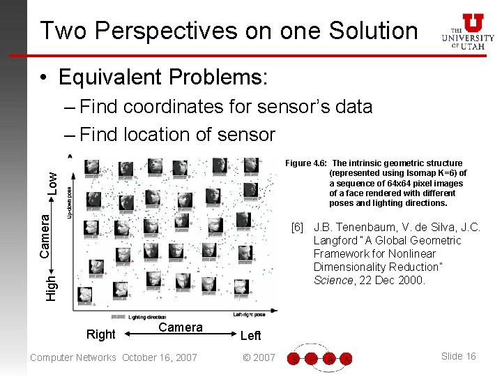
Two Perspectives on one Solution • Equivalent Problems: – Find coordinates for sensor’s data – Find location of sensor Camera Low Figure 4. 6: The intrinsic geometric structure (represented using Isomap K=6) of a sequence of 64 x 64 pixel images of a face rendered with different poses and lighting directions. High [6] J. B. Tenenbaum, V. de Silva, J. C. Langford “A Global Geometric Framework for Nonlinear Dimensionality Reduction” Science, 22 Dec 2000. Right Camera Computer Networks October 16, 2007 Left © 2007 Slide 16
Outline • Manifold Learning and Dimension Reduction • Map-tools Operation • Map-tools Example Computer Networks October 16, 2007 © 2007 Slide 17
Tool Operation • Detailed installation procedure is online: http: //span. ece. utah. edu/pmwiki. php? n=Main. Map-tools • Installation requirements – wnlib – Will Naylor & Bill Chapman, a C code library for computation, data structures – Map-tools code • For use with network data – Flow-tools – Mark Fullmer’s tools for processing Net. Flow data – Net. Flow – Cisco, save 1/N packet headers Computer Networks October 16, 2007 © 2007 Slide 18
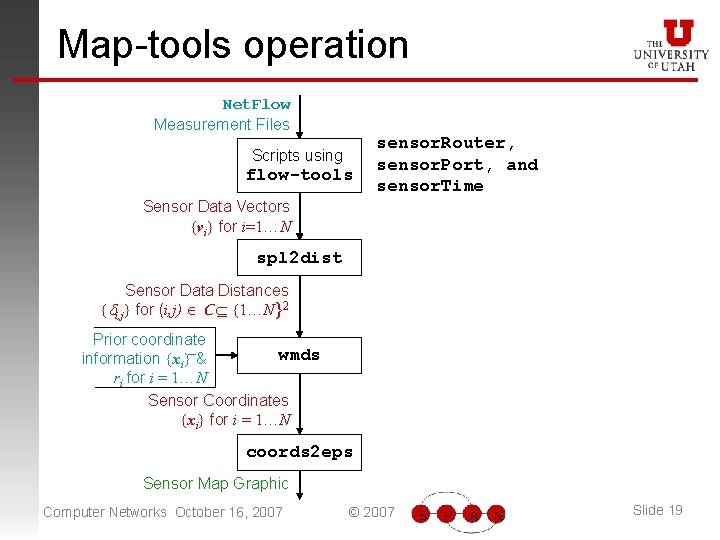
Map-tools operation Net. Flow Measurement Files Scripts using flow-tools sensor. Router, sensor. Port, and sensor. Time Sensor Data Vectors {vi} for i=1…N spl 2 dist Sensor Data Distances {di, j} for (i, j) C {1…N}2 Prior coordinate wmds information {xi} & ri for i = 1…N Sensor Coordinates {xi} for i = 1…N coords 2 eps Sensor Map Graphic Computer Networks October 16, 2007 © 2007 Slide 19
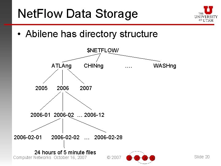
Net. Flow Data Storage • Abilene has directory structure $NETFLOW/ ATLAng CHINng …. WASHng 2005 2006 2007 2006 -01 2006 -02 … 2006 -12 2006 -02 -01 2006 -02 -02 … 2006 -02 -28 24 hours of 5 minute files Computer Networks October 16, 2007 © 2007 Slide 20
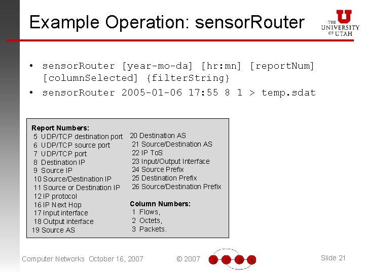
Example Operation: sensor. Router • sensor. Router [year-mo-da] [hr: mn] [report. Num] [column. Selected] {filter. String} • sensor. Router 2005 -01 -06 17: 55 8 1 > temp. sdat Report Numbers: 5 UDP/TCP destination port 6 UDP/TCP source port 7 UDP/TCP port 8 Destination IP 9 Source IP 10 Source/Destination IP 11 Source or Destination IP 12 IP protocol 16 IP Next Hop 17 Input interface 18 Output interface 19 Source AS 20 Destination AS 21 Source/Destination AS 22 IP To. S 23 Input/Output Interface 24 Source Prefix 25 Destination Prefix 26 Source/Destination Prefix Column Numbers: 1 Flows, 2 Octets, 3 Packets. Computer Networks October 16, 2007 © 2007 Slide 21
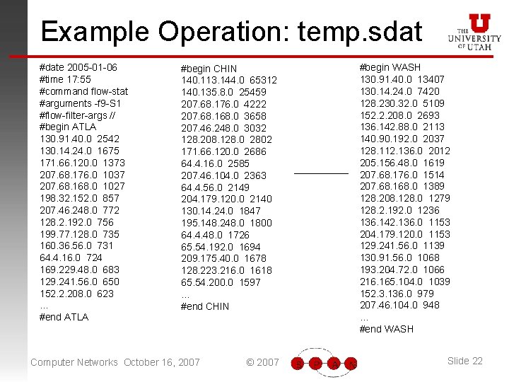
Example Operation: temp. sdat #date 2005 -01 -06 #time 17: 55 #command flow-stat #arguments -f 9 -S 1 #flow-filter-args // #begin ATLA 130. 91. 40. 0 2542 130. 14. 24. 0 1675 171. 66. 120. 0 1373 207. 68. 176. 0 1037 207. 68. 168. 0 1027 198. 32. 152. 0 857 207. 46. 248. 0 772 128. 2. 192. 0 756 199. 77. 128. 0 735 160. 36. 56. 0 731 64. 4. 16. 0 724 169. 229. 48. 0 683 129. 241. 56. 0 650 152. 2. 208. 0 623 … #end ATLA #begin CHIN 140. 113. 144. 0 65312 140. 135. 8. 0 25459 207. 68. 176. 0 4222 207. 68. 168. 0 3658 207. 46. 248. 0 3032 128. 208. 128. 0 2802 171. 66. 120. 0 2686 64. 4. 16. 0 2585 207. 46. 104. 0 2363 64. 4. 56. 0 2149 204. 179. 120. 0 2140 130. 14. 24. 0 1847 195. 148. 248. 0 1800 64. 4. 48. 0 1726 65. 54. 192. 0 1694 209. 175. 40. 0 1678 128. 223. 216. 0 1618 65. 54. 200. 0 1597 … #end CHIN Computer Networks October 16, 2007 © 2007 #begin WASH 130. 91. 40. 0 13407 130. 14. 24. 0 7420 128. 230. 32. 0 5109 152. 2. 208. 0 2693 136. 142. 88. 0 2113 140. 90. 192. 0 2037 128. 112. 136. 0 2012 205. 156. 48. 0 1619 207. 68. 176. 0 1514 207. 68. 168. 0 1389 128. 208. 128. 0 1279 128. 2. 192. 0 1236 136. 142. 136. 0 1153 204. 179. 120. 0 1153 129. 241. 56. 0 1139 130. 91. 56. 0 1068 193. 204. 72. 0 1066 216. 165. 104. 0 1039 152. 3. 136. 0 979 207. 46. 104. 0 948 … #end WASH Slide 22
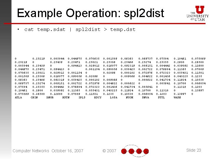
Example Operation: spl 2 dist • cat temp. sdat | spl 2 dist > temp. dst 0 0. 25219 0. 085844 0. 044975 0. 070635 0. 25219 0 0. 25439 0. 25471 0. 25021 0. 085844 0. 25439 0 0. 094413 0. 029012 0. 044975 0. 25471 0. 094413 0 0. 081154 0. 070635 0. 25021 0. 029012 0. 081154 0 0. 081589 0. 25306 0. 016077 0. 090056 0. 02096 0. 06363 0. 25486 0. 092319 0. 058425 0. 080102 0. 069737 0. 25274 0. 089151 0. 082722 0. 072976 0. 07584 0. 25355 0. 084442 0. 076684 0. 072323 0. 10461 0. 2608 0. 039092 0. 11365 0. 055431 0. 075869 0. 26588 0. 12688 0. 07889 0. 11501 ATLA CHIN DNVR HSTN IPLS KSCY Computer Networks October 16, 2007 0. 081589 0. 25306 0. 016077 0. 090056 0. 02096 0 0. 089066 0. 084622 0. 081436 0. 043225 0. 1235 LOSA © 2007 0. 06363 0. 25486 0. 092319 0. 058425 0. 080102 0. 089066 0 0. 088622 0. 041734 0. 11924 0. 10538 NYCM 0. 069737 0. 25274 0. 089151 0. 082722 0. 072976 0. 084622 0. 088622 0 0. 085641 0. 10708 0. 086854 SNVA 0. 07584 0. 25355 0. 084442 0. 076684 0. 072323 0. 081436 0. 041734 0. 085641 0 0. 11318 0. 1203 STTL 0. 10461 0. 2608 0. 039092 0. 11365 0. 055431 0. 043225 0. 11924 0. 10708 0. 11318 0 0. 13997 WASH 0. 075869 0. 26588 0. 12688 0. 07889 0. 11501 0. 1235 0. 10538 0. 086854 0. 1203 0. 13997 0 Slide 23
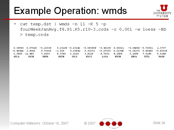
Example Operation: wmds • cat temp. dst | wmds -n 11 -K 5 -p four. Week. Jan. Avg. f 8. S 1. K 5. r 10 -3. crds -r 0. 001 -w loess -ND > temp. crds 0. 34765 0. 87826 -0. 48442 3. 9062 2. 3660 11. 460 ATLA CHIN -0. 15339 0. 75528 7. 2655 DNVR 0. 25189 -0. 25142 -1. 058 0. 25641 6. 7590 2. 1818 HSTN IPLS Computer Networks October 16, 2007 -0. 093909 0. 53271 5. 6226 KSCY © 2007 -0. 45259 -0. 87555 6. 7851 LOSA 0. 80821 0. 22546 4. 1489 NYCM -0. 84686 -0. 73001 -0. 38275 0. 90408 5. 1869 7. 8140 SNVA STTL 1. 3737 -0. 93036 8. 0149 WASH Slide 24
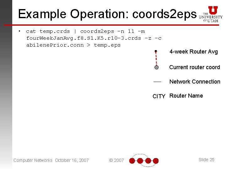
Example Operation: coords 2 eps • cat temp. crds | coords 2 eps -n 11 -m four. Week. Jan. Avg. f 8. S 1. K 5. r 10 -3. crds -z -c abilene. Prior. conn > temp. eps 4 -week Router Avg Current router coord Network Connection CITY Router Name Computer Networks October 16, 2007 © 2007 Slide 25
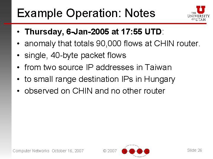
Example Operation: Notes • • • Thursday, 6 -Jan-2005 at 17: 55 UTD: anomaly that totals 90, 000 flows at CHIN router. single, 40 -byte packet flows from two source IP addresses in Taiwan to small range destination IPs in Hungary observed on CHIN and no other router Computer Networks October 16, 2007 © 2007 Slide 26
Outline • Manifold Learning and Dimension Reduction • Map-tools Operation • Map-tools Examples Computer Networks October 16, 2007 © 2007 Slide 27
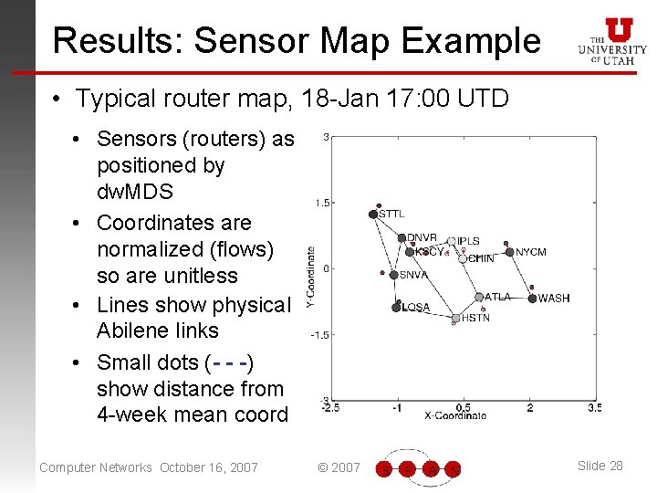
Results: Sensor Map Example • Typical router map, 18 -Jan 17: 00 UTD • Sensors (routers) as positioned by dw. MDS • Coordinates are normalized (flows) so are unitless • Lines show physical Abilene links • Small dots (- - -) show distance from 4 -week mean coord Computer Networks October 16, 2007 © 2007 Slide 28
Maps Respond to Anomaly • Wed. 19 -Jan 2005, 0: 00 -1: 00 UTD • At 0: 30, 0: 35: large network scan – 22, 000 anomalous flows observed at STTL, DNVR, KSCY, IPLS, ATLA – 60 -byte, TCP – From a few Miss. State U. IPs, Src Port < 1024 – To range of Microsoft IPs, Dest Port 113 Computer Networks October 16, 2007 © 2007 Slide 29
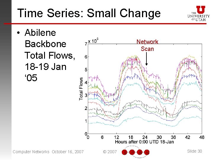
Time Series: Small Change • Abilene Backbone Total Flows, 18 -19 Jan ‘ 05 Computer Networks October 16, 2007 Network Scan © 2007 Slide 30
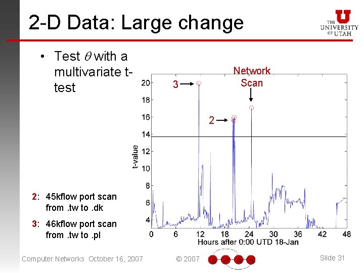
2 -D Data: Large change • Test q with a multivariate ttest Network Scan 3 2 2: 45 kflow port scan from. tw to. dk 3: 46 kflow port scan from. tw to. pl Computer Networks October 16, 2007 © 2007 Slide 31
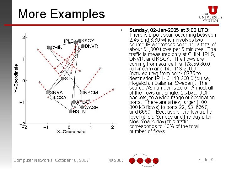
More Examples • Computer Networks October 16, 2007 © 2007 Sunday, 02 -Jan-2005 at 3: 00 UTD: There is a port scan occurring between 2: 45 and 3: 30 which involves two source IP addresses sending a total of about 61, 000 flows per 5 minutes. The traffic is measured only at CHIN, IPLS, DNVR, and KSCY. The flows are coming from source IPs 198. 59. 80. 0 (unknown) and 140. 113. 200. 0 (nctu. edu. tw) from port 48775 to destination IP 140. 113. 200. 0 (du. se, Högskolan Dalarna, Sweden). The source AS number is zero. Almost all of the flows are single, 29 -byte UDP packets, to a wide range of destination ports. There a few, larger (100300 k. B flows) to ports 22, 53, 6667, and 6669. Because of the low traffic level (it is a Sunday and the day after New Year's day) this traffic corresponds to 40% of the total number of flows. Slide 32
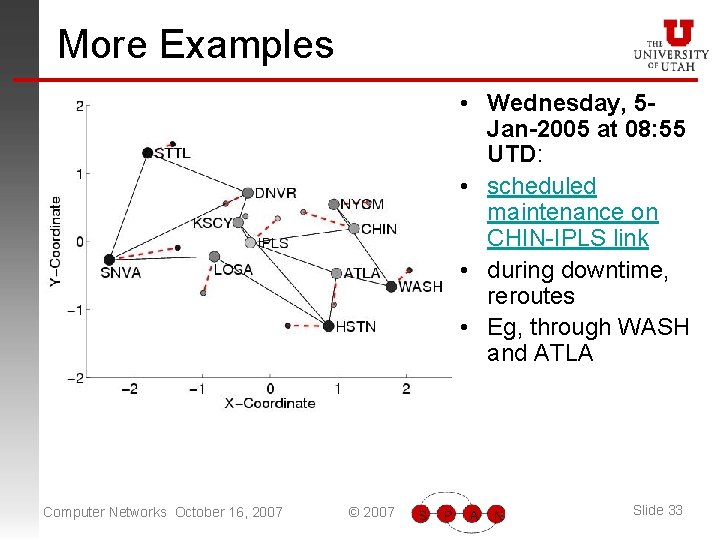
More Examples • Wednesday, 5 Jan-2005 at 08: 55 UTD: • scheduled maintenance on CHIN-IPLS link • during downtime, reroutes • Eg, through WASH and ATLA Computer Networks October 16, 2007 © 2007 Slide 33
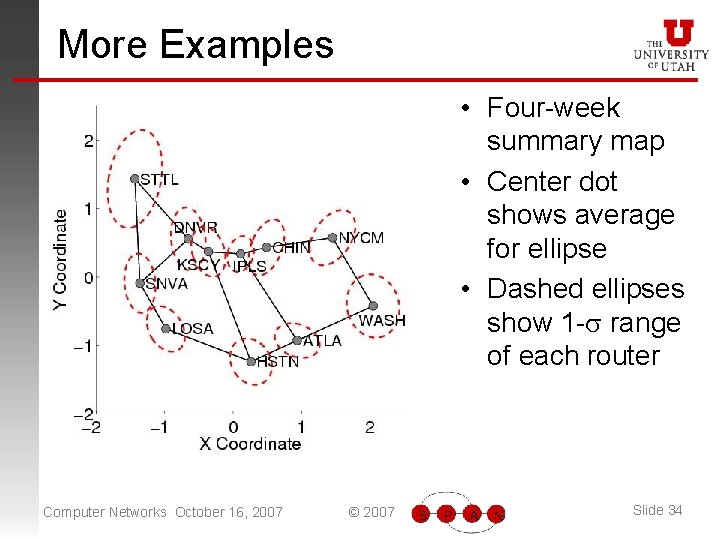
More Examples • Four-week summary map • Center dot shows average for ellipse • Dashed ellipses show 1 -s range of each router Computer Networks October 16, 2007 © 2007 Slide 34
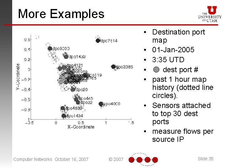
More Examples • Destination port map • 01 -Jan-2005 • 3: 35 UTD • dest port # • past 1 hour map history (dotted line circles). • Sensors attached to top 30 dest ports • measure flows per source IP Computer Networks October 16, 2007 © 2007 Slide 35
Conclusion • We can visualize measurements by their relationship with other measurements – Space, time, feature • One way to do this: – WMDS method, Map-tools Computer Networks October 16, 2007 © 2007 Slide 36