Network Coding Tomography for Network Failures Sidharth Jaggi

Network Coding Tomography for Network Failures Sidharth Jaggi Minghua Chen Hongyi Yao

Computerized Axial Tomography (CAT Scan) 1

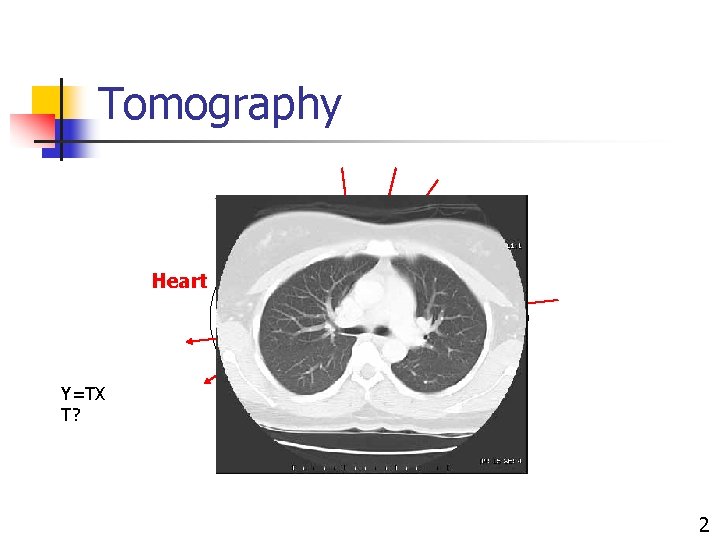
Tomography Heart Y=TX T? 2

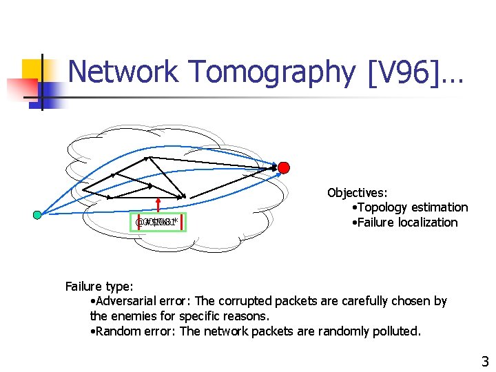
Network Tomography [V 96]… @#$%&* 001001 Objectives: • Topology estimation • Failure localization Failure type: • Adversarial error: The corrupted packets are carefully chosen by the enemies for specific reasons. • Random error: The network packets are randomly polluted. 3

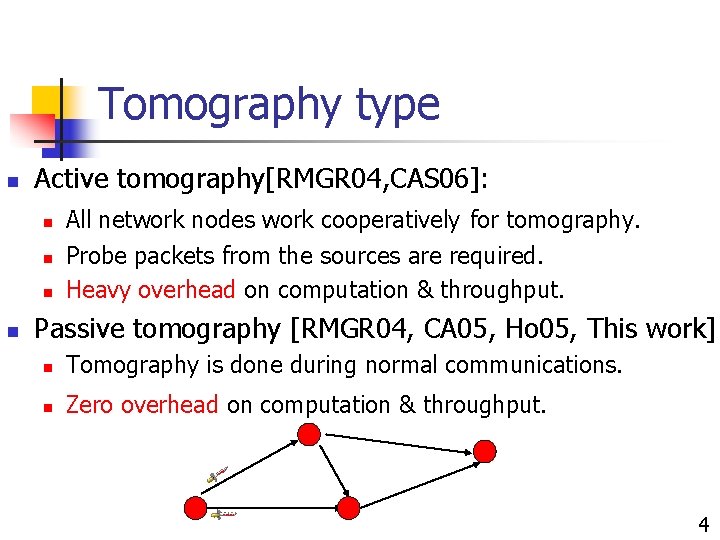
Tomography type n Active tomography[RMGR 04, CAS 06]: n n All network nodes work cooperatively for tomography. Probe packets from the sources are required. Heavy overhead on computation & throughput. Passive tomography [RMGR 04, CA 05, Ho 05, This work]: n Tomography is done during normal communications. n Zero overhead on computation & throughput. 4

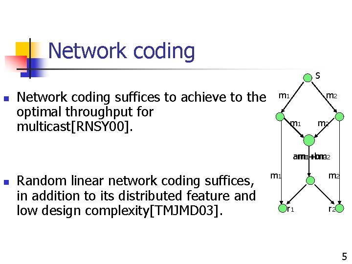
Network coding S n Network coding suffices to achieve to the optimal throughput for multicast[RNSY 00]. m 1 m 2 am m 11+bm +m 2 2 n Random linear network coding suffices, in addition to its distributed feature and low design complexity[TMJMD 03]. m 1 m 2 r 1 r 2 5

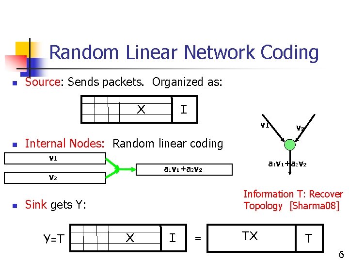
Random Linear Network Coding n Source: Sends packets. Organized as: X I v 1 n Internal Nodes: Random linear coding v 1 Information T: Recover Topology [Sharma 08] Sink gets Y: Y=T a 1 v 1+a 2 v 2 v 2 n v 2 X I = TX T 6

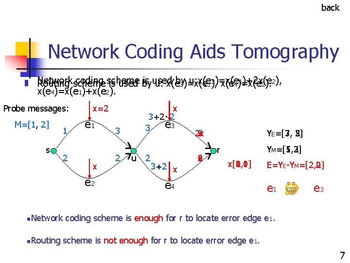
back Network Coding Aids Tomography n n Network coding scheme is used u: x(e 1), 3)=x(e 1)+2 x(e Routing scheme is used by u: x(eby 3)=x(e 4)=x(e 2). 2), x(e 4)=x(e 1)+x(e 2). Probe messages: M=[1, 2] s 1 2 xx=2 e 1 x e 2 n. Network n. Routing x. 3+2 2 e 3 3 3 2 u 2 3+2 x 2 x 7 x 3 5 x 2 0 YE=[7, =[3, 5] 2] YM=[5, 3] =[1, 2] r x[0, 1] x[1, 0] x[2, 1] x[1, 1] e 4 E=YE-YM=[2, 2] =[2, 0] e 1 e 3 coding scheme is enough for r to locate error edge e 1. scheme is not enough for r to locate error edge e 1. 7

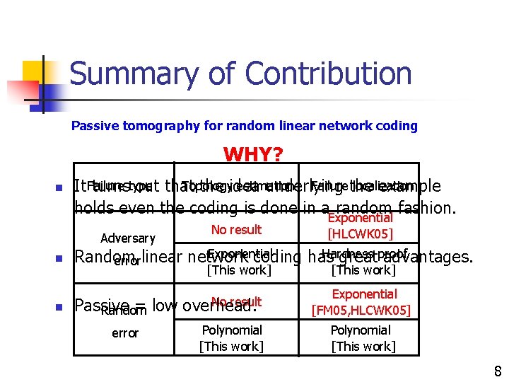
Summary of Contribution Passive tomography for random linear network coding WHY? n Topology estimation Failurethe localization It Failure turnstype out that the idea underlying example holds even the coding is done in a random fashion. Adversary n n No result Exponential [HLCWK 05] Exponential Hardness proof Random errorlinear network coding has great advantages. [This work] Passive = low Random error No result overhead. Polynomial [This work] Exponential [FM 05, HLCWK 05] Polynomial [This work] 8

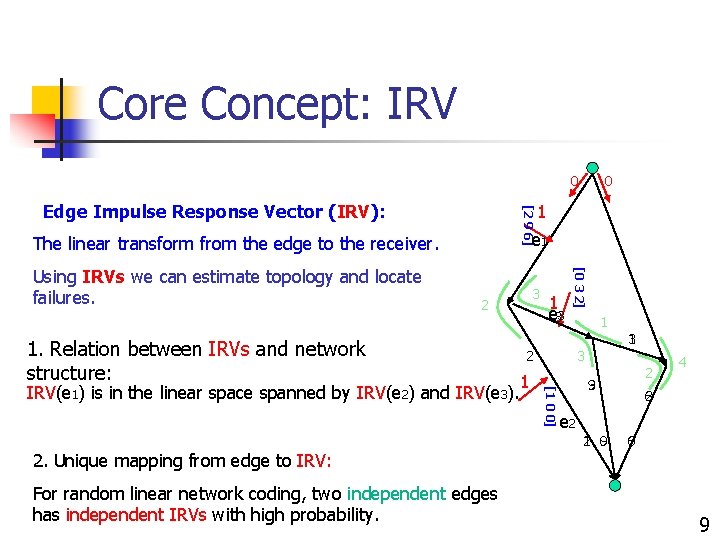
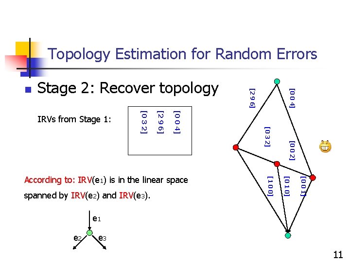
Core Concept: IRV 0 [2 9 6] Edge Impulse Response Vector (IRV): 1 e 1 The linear transform from the edge to the receiver. 3 2 1. Relation between IRVs and network structure: 1 1 3 2 1 3 [1 0 0] IRV(e 1) is in the linear space spanned by IRV(e 2) and IRV(e 3). 1 e 33 [0 3 2] Using IRVs we can estimate topology and locate failures. 0 2 3 9 4 6 2 e 2 1 9 2 0 0 6 2. Unique mapping from edge to IRV: For random linear network coding, two independent edges has independent IRVs with high probability. 9

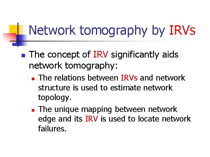
Network tomography by IRVs n The concept of IRV significantly aids network tomography: n n The relations between IRVs and network structure is used to estimate network topology. The unique mapping between network edge and its IRV is used to locate network failures.

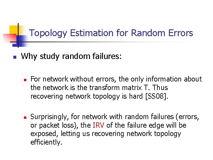
Topology Estimation for Random Errors n Why study random failures: n n For network without errors, the only information about the network is the transform matrix T. Thus recovering network topology is hard [SS 08]. Surprisingly, for network with random failures (errors, or packet loss), the IRV of the failure edge will be exposed, letting us recovering network topology efficiently.

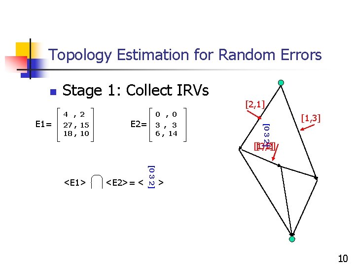
Topology Estimation for Random Errors n Stage 1: Collect IRVs 4 , 2 27 , 15 18 , 10 0 , 0 E 2= 3 , 3 6 , 14 [1, 3] [0 3 2] E 1= [2, 1] [1, 1] [3, 2] <E 2>= < [0 3 2] <E 1> > 10

Topology Estimation for Random Errors [0 0 2] [0 0 1] [0 1 0] spanned by IRV(e 2) and IRV(e 3). [1 0 0] According to: IRV(e 1) is in the linear space [0 3 2] [0 0 4] [2 9 6] [0 3 2] IRVs from Stage 1: [0 0 4] Stage 2: Recover topology [2 9 6] n e 1 e 2 e 3 11

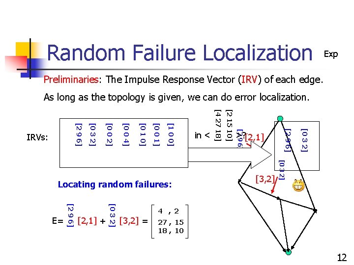
Random Failure Localization Exp Preliminaries: The Impulse Response Vector (IRV) of each edge. As long as the topology is given, we can do error localization. [0 3 2] [3, 2] [0 3 2] >? [2, 1] [2 9 6] [2, 1] + [0 3 2] [2 9 6] E= [2 15 10] Locating random failures: in < [4 27 18] [1 0 0] [0 0 1] [0 1 0] [0 0 4] [0 0 2] [0 3 2] [2 9 6] IRVs: 4 , 2 [3, 2] = 27 , 15 18 , 10 12

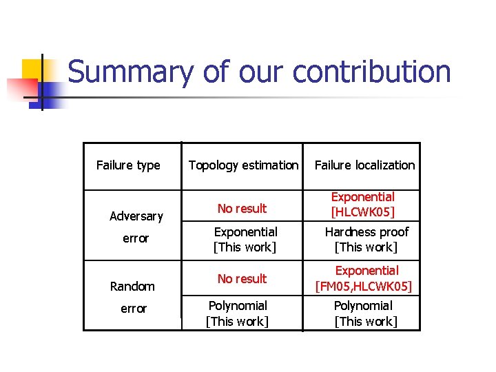
Summary of our contribution Failure type Adversary error Random error Topology estimation Failure localization No result Exponential [HLCWK 05] Exponential [This work] Hardness proof [This work] No result Exponential [FM 05, HLCWK 05] Polynomial [This work]

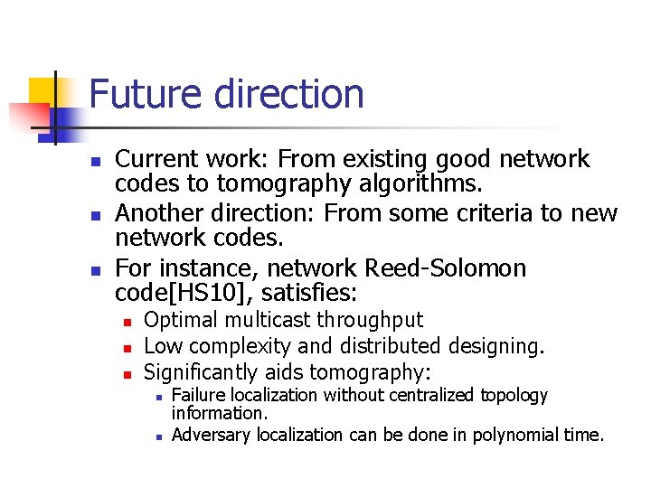
Future direction n Current work: From existing good network codes to tomography algorithms. Another direction: From some criteria to new network codes. For instance, network Reed-Solomon code[HS 10], satisfies: n n n Optimal multicast throughput Low complexity and distributed designing. Significantly aids tomography: n n Failure localization without centralized topology information. Adversary localization can be done in polynomial time.

Related works

Network Coding Tomography for Network Failures n Thanks! n Questions? Details in: Hongyi Yao and Sidharth Jaggi and Minghua Chen, Network Tomography for Network Failures, under submission to IEEE Trans. on Information Theory, and arxiv: 0908 -0711 14