Nave Bayes Classifier Ke Chen Outline Background Probability
Naïve Bayes Classifier Ke Chen
Outline • Background • Probability Basics • Probabilistic Classification • Naïve Bayes – Principle and Algorithms – Example: Play Tennis • Zero Conditional Probability • Summary 2
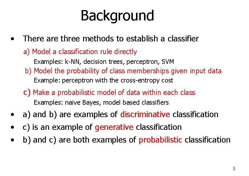
Background • There are three methods to establish a classifier a) Model a classification rule directly Examples: k-NN, decision trees, perceptron, SVM b) Model the probability of class memberships given input data Example: perceptron with the cross-entropy cost c) Make a probabilistic model of data within each class Examples: naive Bayes, model based classifiers • a) and b) are examples of discriminative classification • c) is an example of generative classification • b) and c) are both examples of probabilistic classification 3
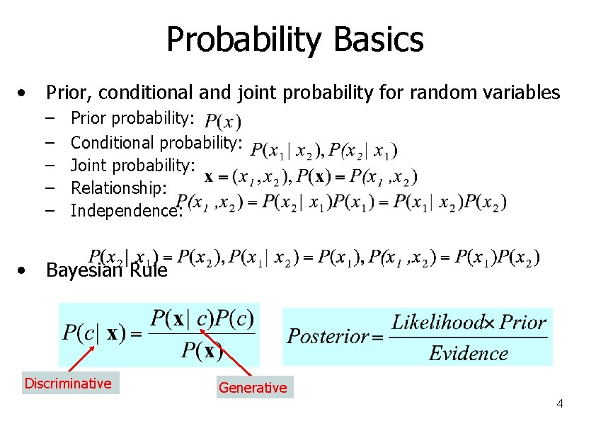
Probability Basics • Prior, conditional and joint probability for random variables – – – • Prior probability: Conditional probability: Joint probability: Relationship: Independence: Bayesian Rule Discriminative Generative 4
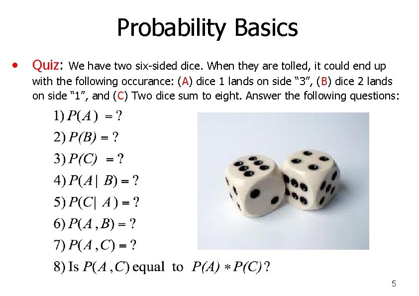
Probability Basics • Quiz: We have two six-sided dice. When they are tolled, it could end up with the following occurance: (A) dice 1 lands on side “ 3”, (B) dice 2 lands on side “ 1”, and (C) Two dice sum to eight. Answer the following questions: 5
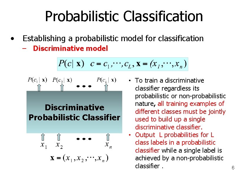
Probabilistic Classification • Establishing a probabilistic model for classification – Discriminative model Discriminative Probabilistic Classifier • To train a discriminative classifier regardless its probabilistic or non-probabilistic nature, all training examples of different classes must be jointly used to build up a single discriminative classifier. • Output L probabilities for L class labels in a probabilistic classifier while a single label is achieved by a non-probabilistic classifier. 6
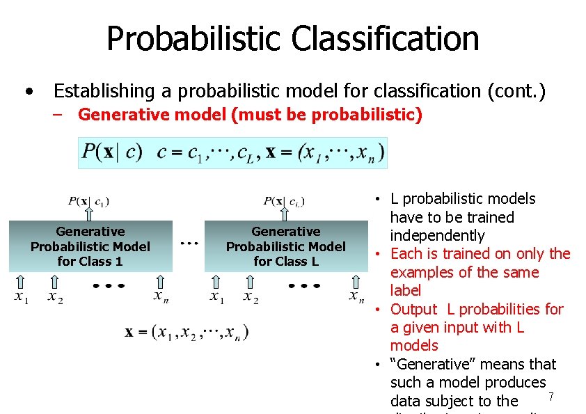
Probabilistic Classification • Establishing a probabilistic model for classification (cont. ) – Generative model (must be probabilistic) Generative Probabilistic Model for Class 1 Generative Probabilistic Model for Class L • L probabilistic models have to be trained independently • Each is trained on only the examples of the same label • Output L probabilities for a given input with L models • “Generative” means that such a model produces 7 data subject to the
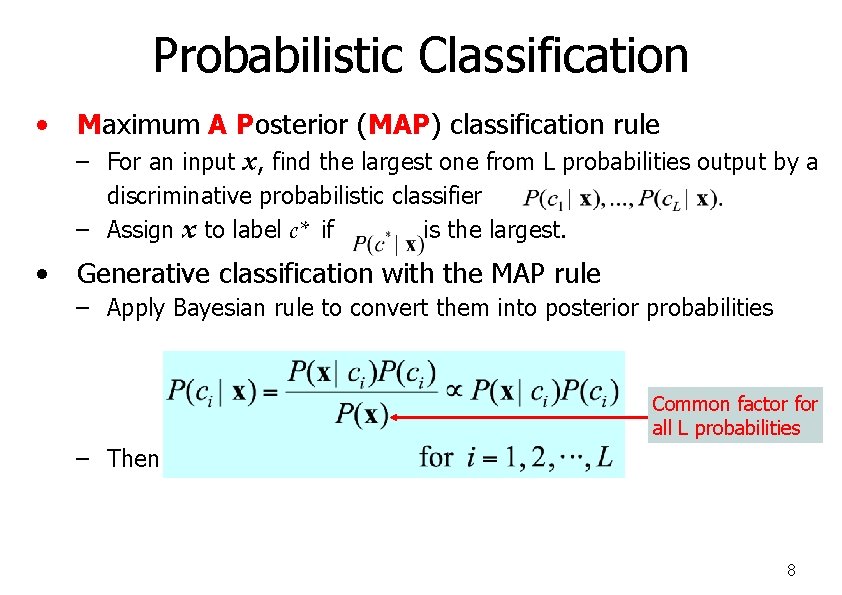
Probabilistic Classification • Maximum A Posterior (MAP) classification rule – For an input x, find the largest one from L probabilities output by a discriminative probabilistic classifier – Assign x to label c* if is the largest. • Generative classification with the MAP rule – Apply Bayesian rule to convert them into posterior probabilities Common factor for all L probabilities – Then apply the MAP rule to assign a label 8
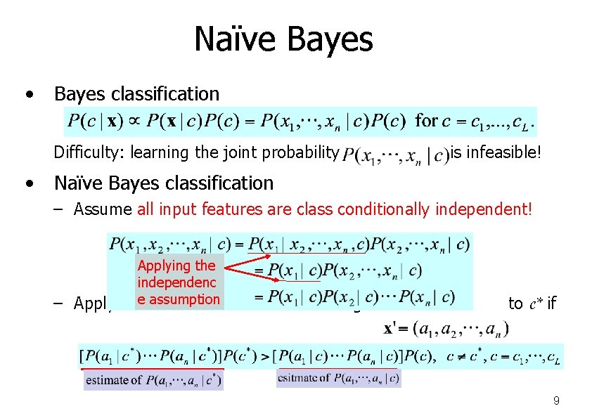
Naïve Bayes • Bayes classification Difficulty: learning the joint probability • is infeasible! Naïve Bayes classification – Assume all input features are class conditionally independent! – Applying the independenc assumption thee MAP classification rule: assign to c* if 9

Naïve Bayes 10
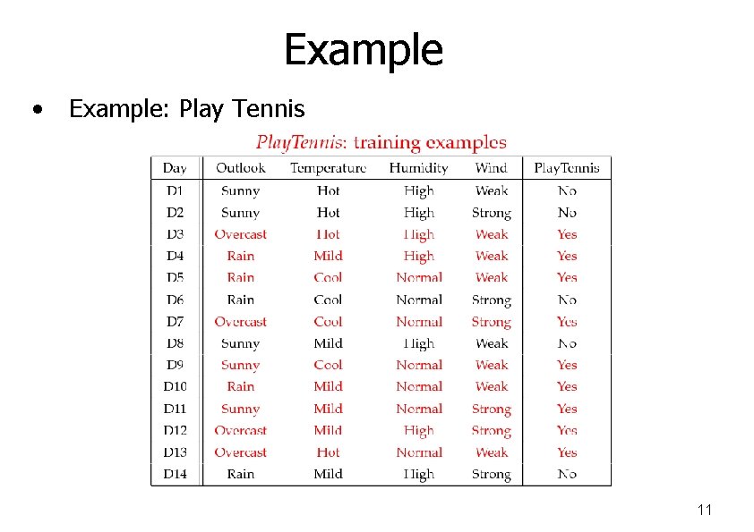
Example • Example: Play Tennis 11
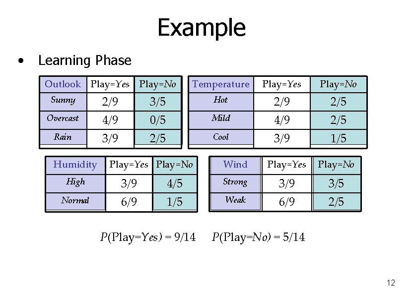
Example • Learning Phase Outlook Play=Yes Play=No Temperature Play=Yes Play=No Sunny 2/9 3/5 Hot 2/9 2/5 Overcast 4/9 0/5 Mild 4/9 2/5 Rain 3/9 2/5 Cool 3/9 1/5 Humidity Play=Yes Play=No Wind Play=Yes Play=No High 3/9 4/5 Strong 3/9 3/5 Normal 6/9 1/5 Weak 6/9 2/5 P(Play=Yes) = 9/14 P(Play=No) = 5/14 12
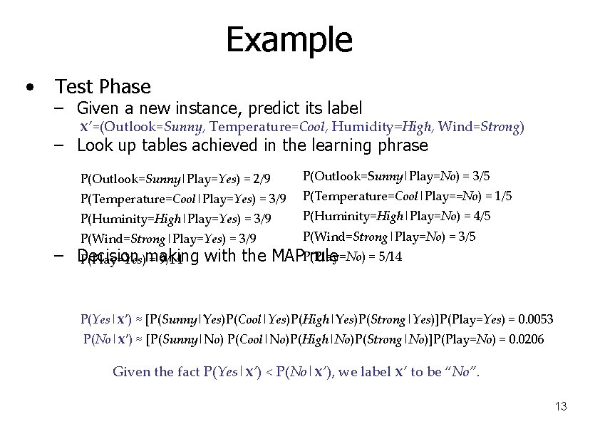
Example • Test Phase – Given a new instance, predict its label x’=(Outlook=Sunny, Temperature=Cool, Humidity=High, Wind=Strong) – Look up tables achieved in the learning phrase P(Outlook=Sunny|Play=Yes) = 2/9 P(Temperature=Cool|Play=Yes) = 3/9 P(Huminity=High|Play=Yes) = 3/9 P(Wind=Strong|Play=Yes) = 3/9 P(Outlook=Sunny|Play=No) = 3/5 P(Temperature=Cool|Play==No) = 1/5 P(Huminity=High|Play=No) = 4/5 P(Wind=Strong|Play=No) = 3/5 = 5/14 – Decision with the MAPP(Play=No) rule P(Play=Yes)making = 9/14 P(Yes|x’) ≈ [P(Sunny|Yes)P(Cool|Yes)P(High|Yes)P(Strong|Yes)]P(Play=Yes) = 0. 0053 P(No|x’) ≈ [P(Sunny|No) P(Cool|No)P(High|No)P(Strong|No)]P(Play=No) = 0. 0206 Given the fact P(Yes|x’) < P(No|x’), we label x’ to be “No”. 13
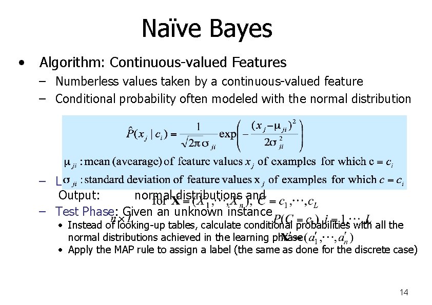
Naïve Bayes • Algorithm: Continuous-valued Features – Numberless values taken by a continuous-valued feature – Conditional probability often modeled with the normal distribution – Learning Phase: Output: normal distributions and – Test Phase: Given an unknown instance • Instead of looking-up tables, calculate conditional probabilities with all the normal distributions achieved in the learning phrase • Apply the MAP rule to assign a label (the same as done for the discrete case) 14
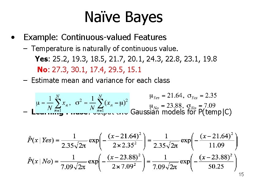
Naïve Bayes • Example: Continuous-valued Features – Temperature is naturally of continuous value. Yes: 25. 2, 19. 3, 18. 5, 21. 7, 20. 1, 24. 3, 22. 8, 23. 1, 19. 8 No: 27. 3, 30. 1, 17. 4, 29. 5, 15. 1 – Estimate mean and variance for each class – Learning Phase: output two Gaussian models for P(temp|C) 15
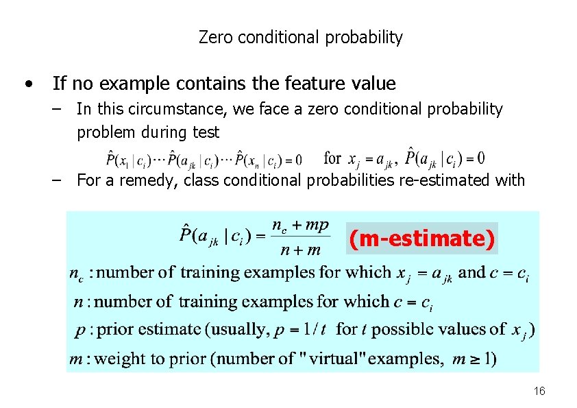
Zero conditional probability • If no example contains the feature value – In this circumstance, we face a zero conditional probability problem during test – For a remedy, class conditional probabilities re-estimated with (m-estimate) 16
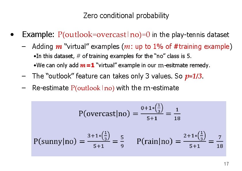
Zero conditional probability • Example: P(outlook=overcast|no)=0 in the play-tennis dataset – Adding m “virtual” examples (m: up to 1% of #training example) • In this dataset, # of training examples for the “no” class is 5. • We can only add m=1 “virtual” example in our m-esitmate remedy. – The “outlook” feature can takes only 3 values. So p=1/3. – Re-estimate P(outlook|no) with the m-estimate 17
Summary • Naïve Bayes: the conditional independence assumption – Training and test are very efficient – Two different data types lead to two different learning algorithms – Working well sometimes for data violating the assumption! • A popular generative model – Performance competitive to most of state-of-the-art classifiers even in presence of violating independence assumption – Many successful applications, e. g. , spam mail filtering – A good candidate of a base learner in ensemble learning – Apart from classification, naïve Bayes can do more… 18
- Slides: 18